Ch16 The Market of Labor
Labor Supply Model
縱軸為 C consumption(等同於 income,好東西),橫軸為 L working hours(壞東西)
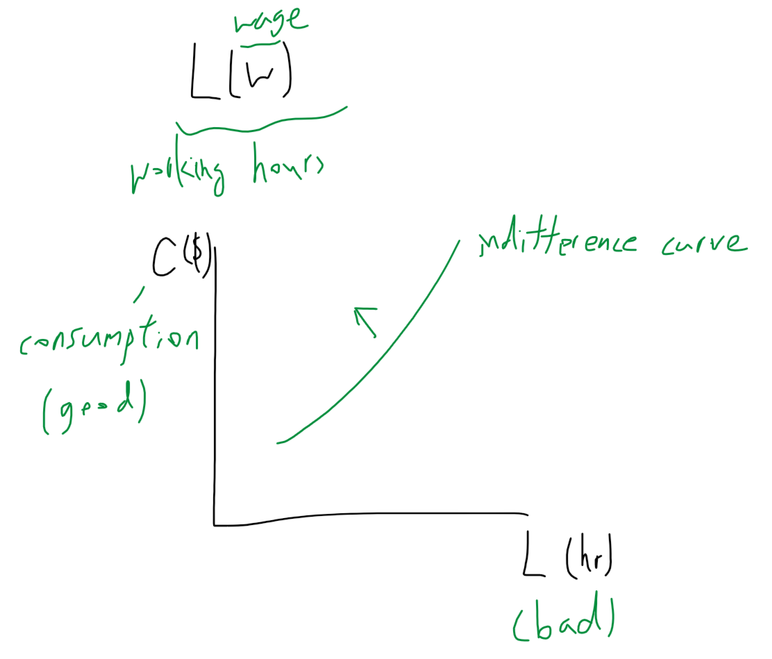
C~0~ 為非勞工性質之收入(non-labor income,如股票、出租房子等) C~0~ 上升 → income effect → leisure 增加 i.e. L 下降 at some point, L 下降到 0,表此人不再為"工資"而工作(可為其他東如西興趣工作)
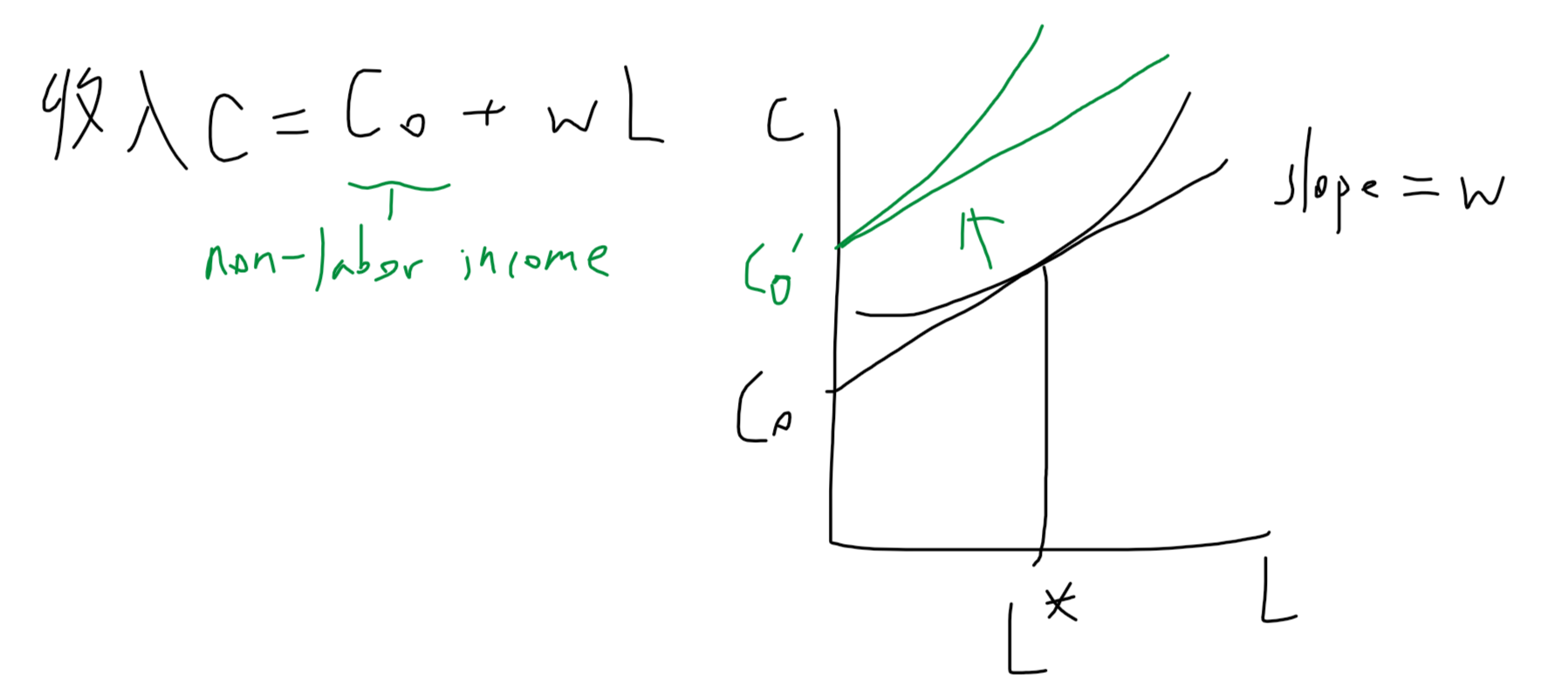
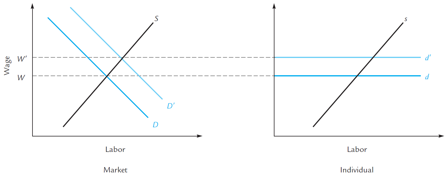
an increase in nonlabor income
若是只有一個人 nonlabor income 上升 → individual supply curve 左移(上移) → 工時減少

若是整個 market 的勞工一起 nonlabor income 上升 → market supply curve 左移 → wage 上升
→ individual 工時可能上升可能減少 (但 market labor supply 必減少)
Changes in Productivity
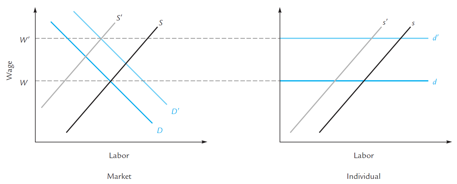
若 individual\(MP_L\) 上升
→ \(\text{MRP}_L\) 上升 → demand 上升
→ wage 上升 & quantity of labor supply 上升
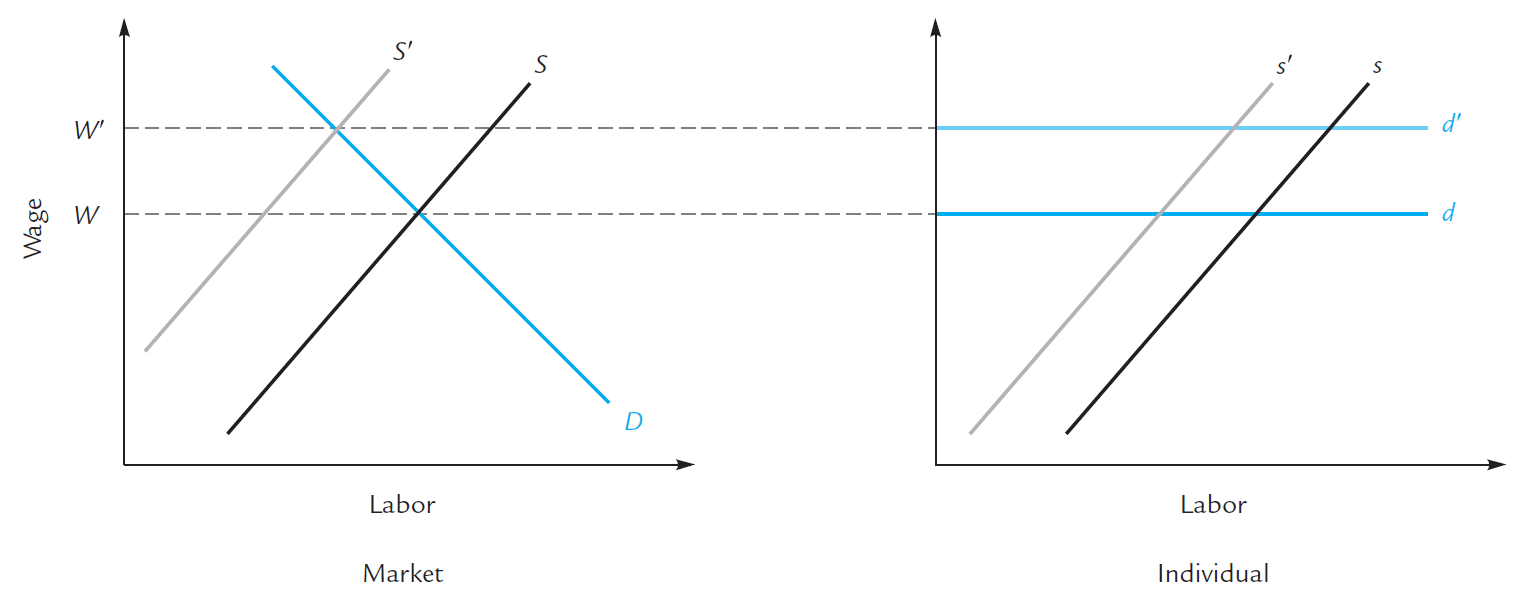
但若是整個 market 的 \(\text{MRP}_L\) 上升
→ 資產價值上升(因為資產跟人的價值有關) → labor's nonlabor income 上升
→ individual supply curve 左移 → market supply curve 左移
→ wage 上升但 quantity of labor supply 不一定
Intertemporal Substitution
若需求(productibity)的增加只是短期性的(e.g. 1989 Alaska oil spill)
→ individual labor 更想工作 → supply curve 左移
→ market supply curve 左移 while demand curve 右移
→ wage 可能上升可能下降(但下降不合理)
→ 工時大量增加但 wage 可能沒上升那麼多 due to
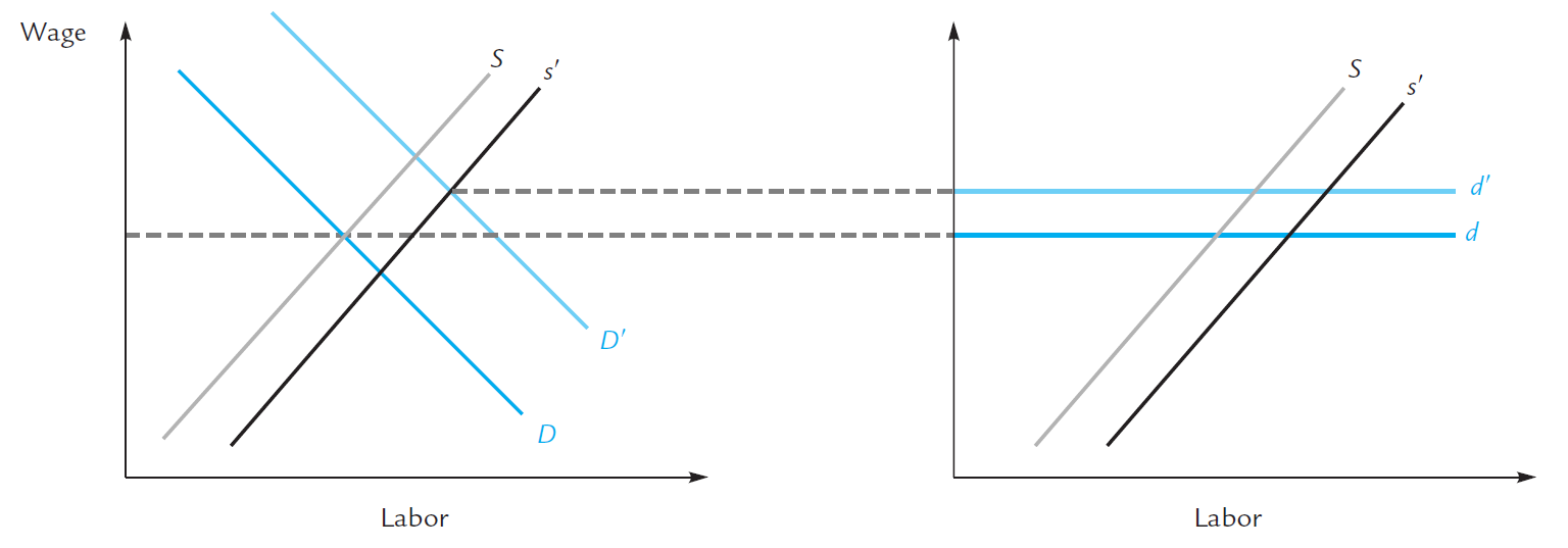
a temporary increase in productivity has much higher effect then a permanent one
Unemployment
設政府保證 I' 之收入
設固定工資
I' = w x L'
for those whose L* < L' before subsidy → choose L=0(工作與否都領 I')
for those whose L* > L' before subsidy
-
choose L=L → L=L, c=I*
-
choose L=0 → L=0 < L ^better^, c=I' < I ^worse^
may choose the latter i.e. L=0
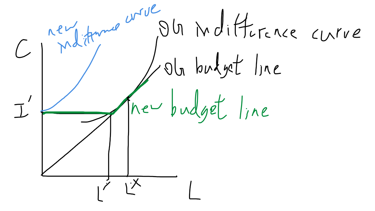
結論:鼓勵部份人民失業(原本收入小於保障收入&原本收入沒有比保障收入高很多者)
Labor Supply Change when Wage Rise
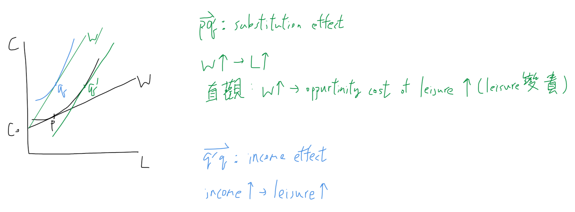
工資上漲
- substitution effect (綠):working hour 增加 i.e. leisure 減少 due to leisure 漲價
- income effect (藍):working hour 減少 i.e. 買更多 leisure
哪個比較大?
實證發現:
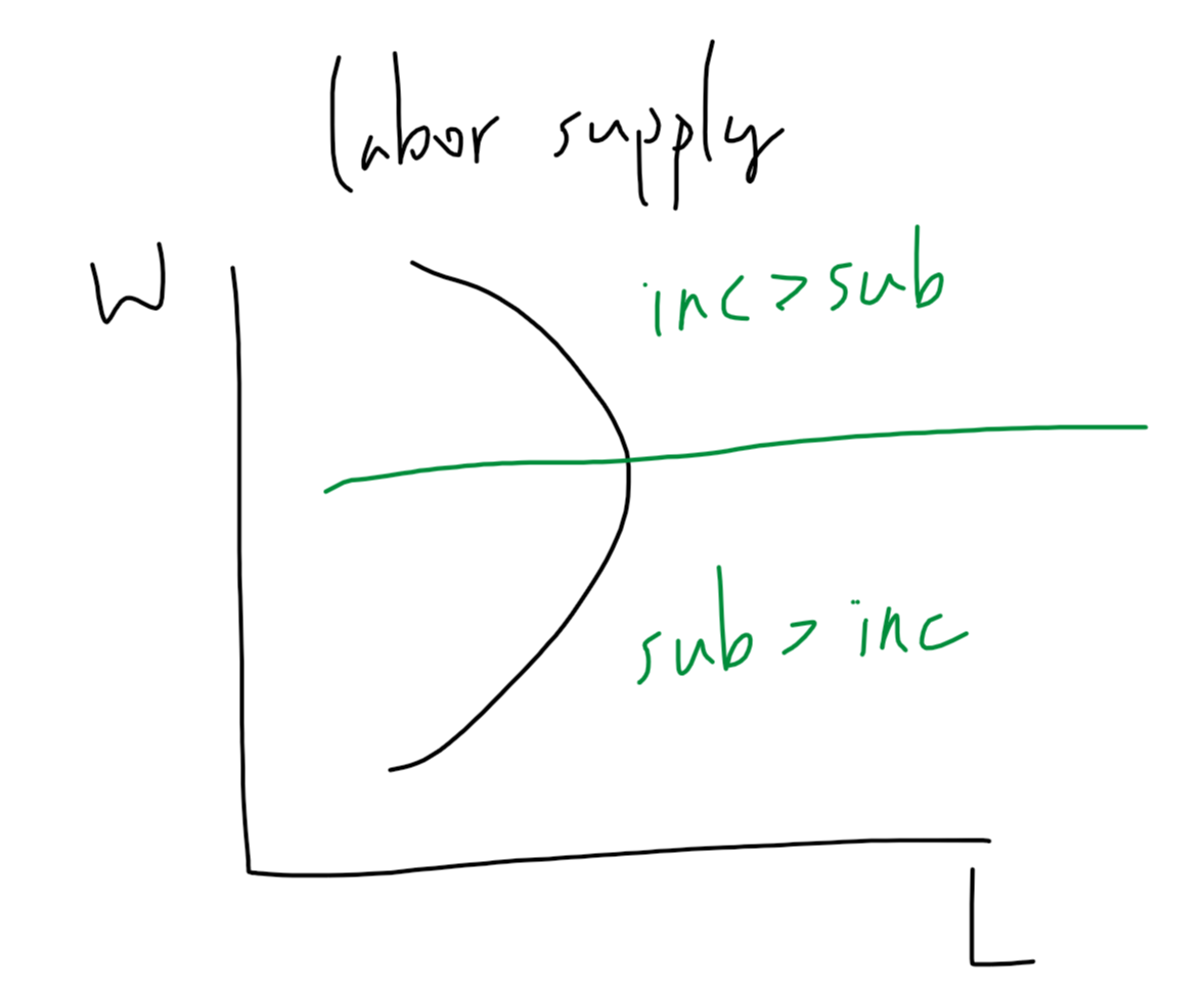
when wage rises, ppl with low wage experience little income effect ,
while ppl with high wages experience great income effect
→ 上圖
見 HW P9.
實例:
US implement medical insurance
→ 醫療變便宜
→ 醫療 demand 增加
→ nurse demand 增加
→ wage of nurse 增加
→ avg nurse's working hours 減少
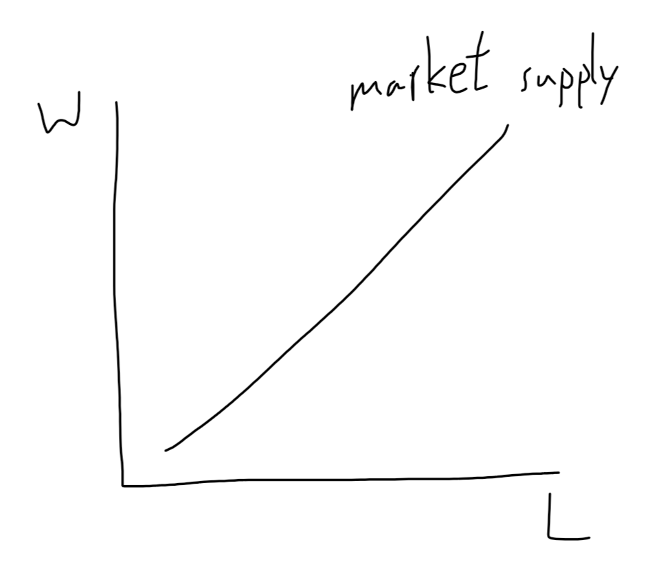
BUTT, 更多 nurse 進入市場 due to wage of nurse rise
→ with the rise of wage, market supply of labor 增加 despite individual supply of labor 下降
1890 vs. 1990
工業革命初期勞工工時長工資少,而今日則是工時短工資高,符合上面 backward-bending 的現象
但也有可能是因為今日的 nonlabor income 增加 → 理想工作的時數變短
工資差異
補償性工資
如 106 台北清潔人員 40k
human goods 人力資本
投資自己
如進修 → 增加自己的 human capital
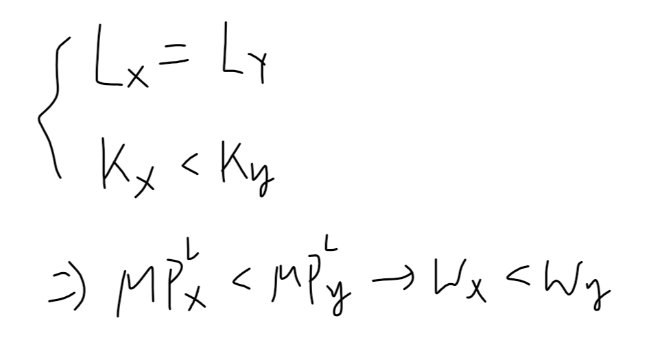
\(MP_L\) and capital gooㄕㄨㄕㄨds
labor move
機器設備 capital 較好 → 勞工生產力 \(MP_L\) 較高 與 capital goods 為 complementary goods 互補品
capital 多 → \(MP_L\) 高 → \(MRP_L\) 高 又 wage = \(MRP_L\) = \(P \times MP_L\)
已知 labor 變多 →\(MP_L\) 下降
→ labor 會一直從資本多,\(MP_L\) 高的國家地方移動到資本少,\(MP_L\) 低的地方,直到兩地\(MP_L\) 相等
但是勞工會有移動限制
capital move
設有 x、y 兩國,兩者勞工數相等但 capital 數不等,造成邊際產出差異
已知 capital 愈高,capital 的邊際產出愈低
so 商人會把 capital 從 capital 較多,勞工邊際產出較高之國,移動到 capital 較少,勞工邊際產出較低之國
直到兩國之 capital 數量相等,勞工邊際產出也相等(labor 數量一直相同)
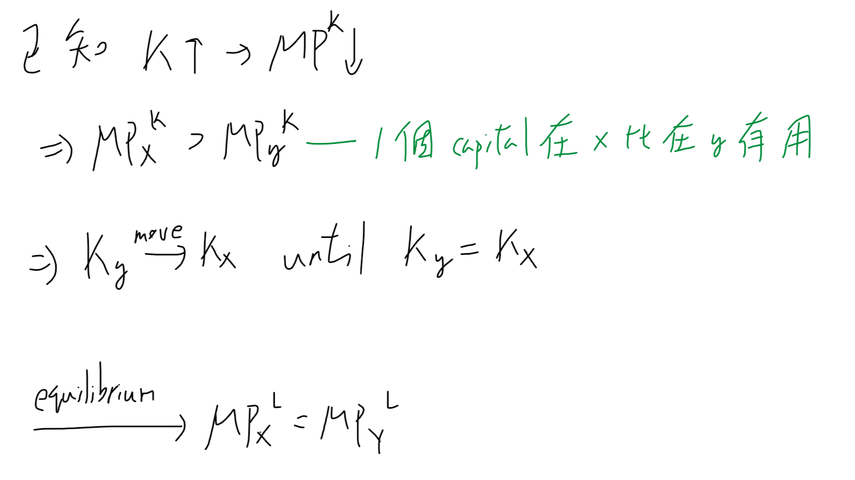
但是這也不符和實際世界情況,不同國家間仍存在\(MP_L\) 差異
此乃經濟學之
unsolved mystery
HW
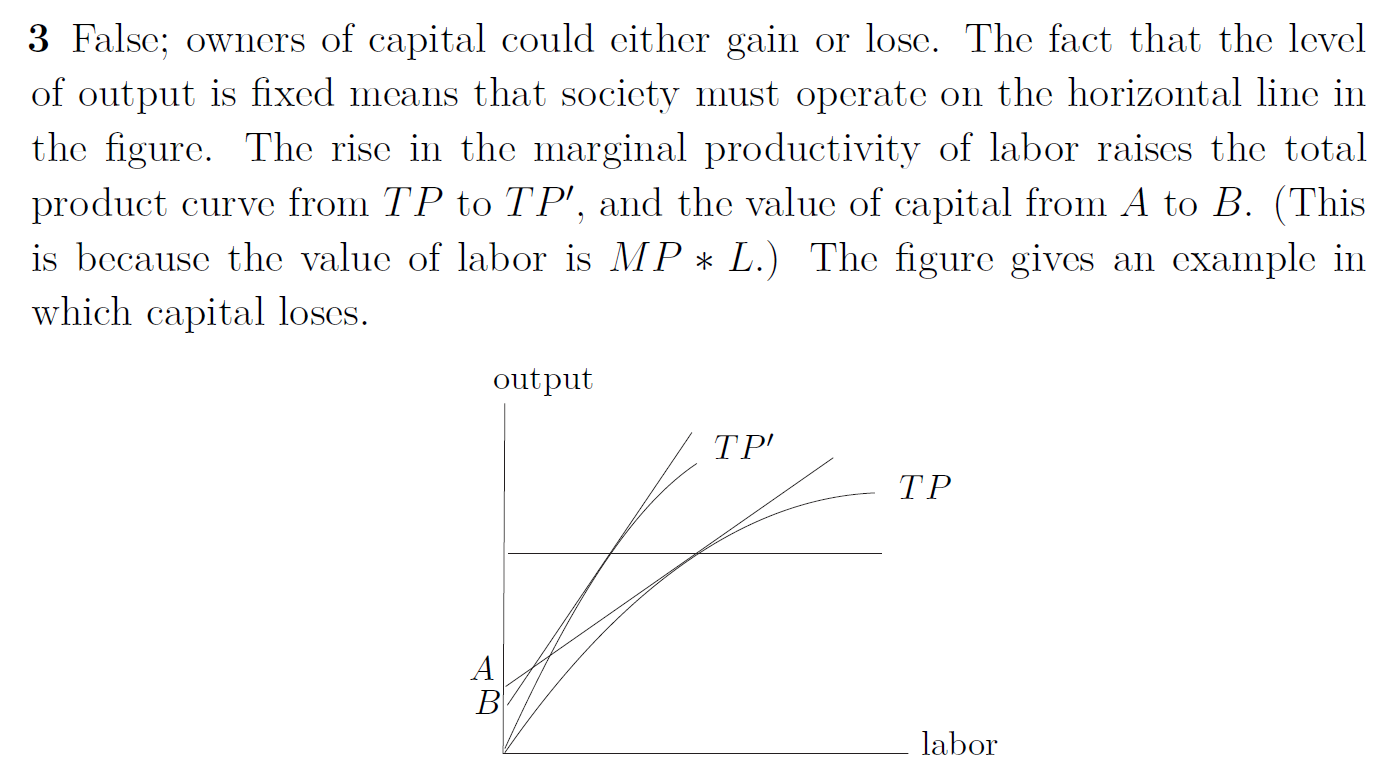
P3
P9 !!!

False, the former man experience both substutution effect & income effect, while the latter experience very little income effect
→ the man with most of his income from wages may works more or works less due to sub effect - income effect,
while the man with most of his income from nonlabor income works more due to sub effect
P15 !!!