Algorithms
resources
Solutions to Introduction to Algorithms Third Edition
pseudocode
- array position 1-A.length
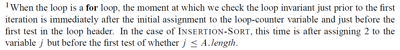
- for
for i = 1 to A.length
loop invariant
- está verda siempre
- pre, peri & post loop iteration
- like math induction
- 3 properties
- initialization
- in for loop, just after the assignment of i, before the boolean test
- maintenance
- termination
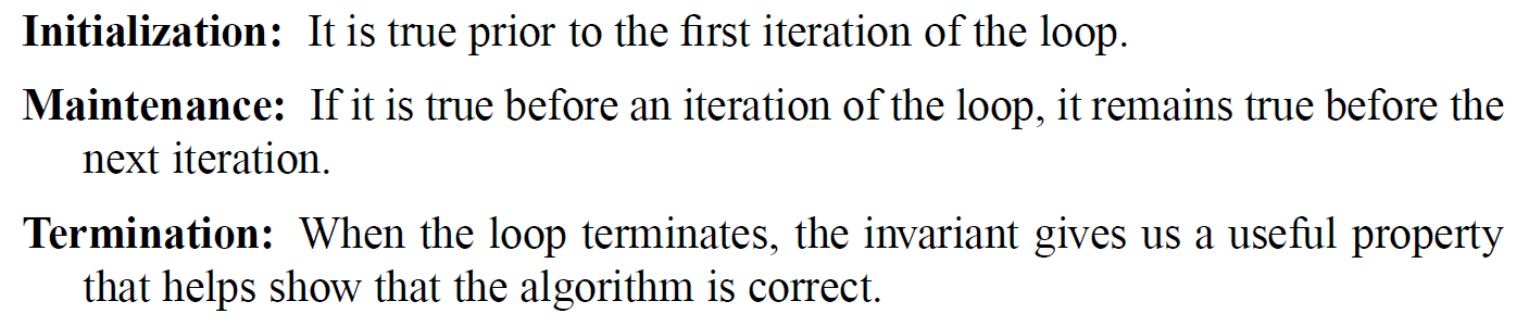
- initialization
complexity
- time complexity
- steps
- space complexity
- memory requirement
functions
- f(n)
- \(f(n) \geq 0\) nonnegative
- \(n \in N\)
- \(f(n)=O(g(n))\)
- upper bound
- \(\exists c>0\) and \(n_0>0\) s.t. \(0\leq f(n)\leq cg(n)\) \(\forall n \geq n_0\)
- \(\lim_{n\rightarrow\infty} \frac{f(n)}{g(n)} \in [0,\infty)(i.e. <\infty)\) if the limit exists
- \(f(n)= \Omega(g(n))\)
- lower bound
- \(\exists c>0\) and \(n_0>0\) s.t. \(0\leq cg(n)\leq f(n)\) \(\forall n \geq n_0\)
- \(\lim_{n\rightarrow\infty} \frac{f(n)}{g(n)} \in (0,\infty](i.e. >0)\) if the limit exists
- \(f(n)=\Theta(g(n))\)
- tight bound, bounded by \(O\) & \(\Omega\)
- \(f(n)=O(g(n))\) and \(f(n)= \Omega(g(n))\)
- \(\exists c_1,c_2>0\) and \(n_0>0\) s.t. \(0\leq c_1g(n) \leq f(n)\leq c_2g(n)\) \(\forall n \geq n_0\)
- \(\lim_{n\rightarrow\infty} \frac{f(n)}{g(n)} \in (0,\infty)\) if the limit exists
- \(f(n)=o(g(n))\)
- untightly upper bound
- \(\forall c>0\) , \(\exists n_0>0\) s.t. \(0\leq f(n)< cg(n)\) \(\forall n \geq n_0\)
- \(\lim_{n\rightarrow\infty} \frac{f(n)}{g(n)} = 0\) if the limit exists
- \(f(n)= \omega(g(n))\)
- untightly lower bound
- \(\forall c>0\) , \(\exists n_0>0\) s.t. \(0\leq cg(n)< f(n)\) \(\forall n \geq n_0\)
- \(\lim_{n\rightarrow\infty} \frac{f(n)}{g(n)} = \infty\) if the limit exists
properties
- transitivity
- \(f(n)=\Pi(g(n))\) and \(g(n)=\Pi(h(n))\) → \(f(n)=\Pi(h(n))\) for \(\Pi=everything\)
- rule of sums
- \(f(n)+g(n)=\Pi(max\{f(n),g(n)\})\) for \(\Pi=big\)
- rule of products
- \(f_1(n)=\Pi(g_1(n))\) and \(f_2(n)=\Pi(g_2(n))\) → \(f_1(n)f_2(n)=\Pi(g_1(n)g_2(n))\) for \(\Pi=everything\)
- transpose symmetry
- \(f(n)=O(g(n))\iff g(n)=\Omega(f(n))\)
- \(f(n)=o(g(n))\iff g(n)=\omega(f(n))\)
- reflexivity
- \(f(n)=\Pi(f(n))\) for \(\Pi=big\)
- symmetry
- \(f(n)=\Theta(g(n))\iff g(n)=\Theta(f(n))\)
notation
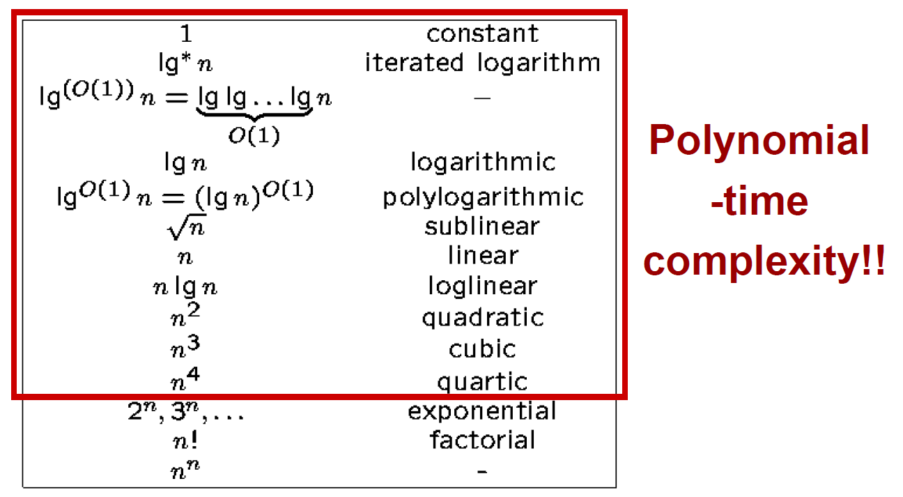
- \(lgn = log_2n\)
- \(lg^{(i)}n = lglglglg....lgn\)
- \(lg^*n=min\{i\geq0:lg^in\leq1\}\)
- polynomial-time
- \(O(p(n))\), \(p(n)=n^{O(1)}\)
others
- input size: size of encoded binary string
- integer n → input size = lgn
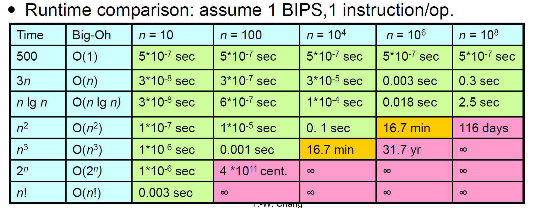
- BIPS
- billion instruction/operation per second
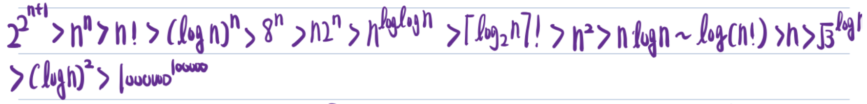
growth of function examples
- ratio limit doesn't exist
- \(f(n)=2^n\)
- \(g(n)=2^n\) if n is even, \(g(n)=2^{n-1}\) otherwise

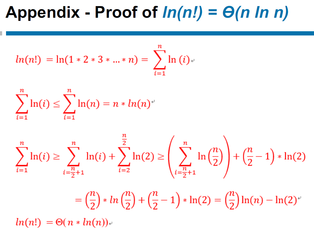
- Stirling's approximation
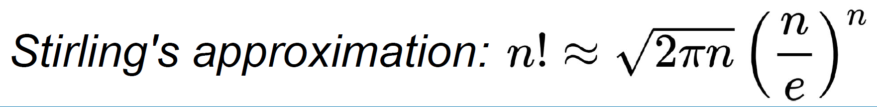
- can use it to approximate \((lgn)!\in\Theta(n^{lg(lgn)})>n^k\)
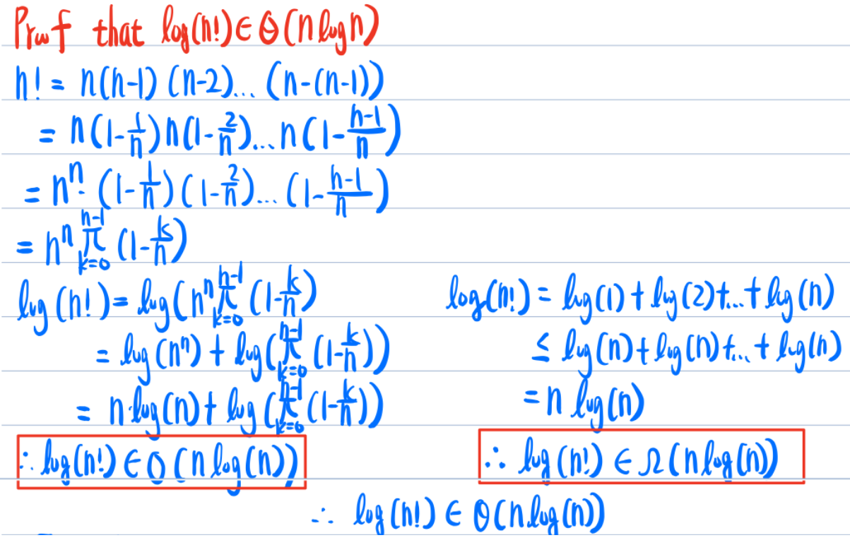
- \(ln(n!)\in \Theta(nlnn)\)
Divide and Conquer
- divide into subproblems
- conquer subproblems recursively
- combine the subsolutions into an overall solution
mathematical induction
- weak induction
- basis step
- inductive step
- \(P(K) → P(K+1)\) \(\forall k\in N\)
- strong induction
- basis step
- inductive step
- \(P(0)\land P(1)\land .... \land P(K) → P(K+1)\) \(\forall k\in N\)
- 跟 weak induction 一樣強
- 比較好證
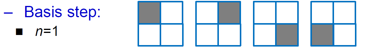
- defective chessboard
- \(2^n\times2^n\) 缺一塊的 chessboard 可被 triominoes 拼完
- basis step
- inductive step
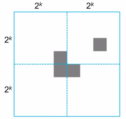
- 中間挖一個 triomonoe 洞,變成四塊缺一角的 \(2^{k-1}\times 2^{k-1}\) 的 chessboard
- so 假設 k-1 成立,則 k 必成立
solve recurence
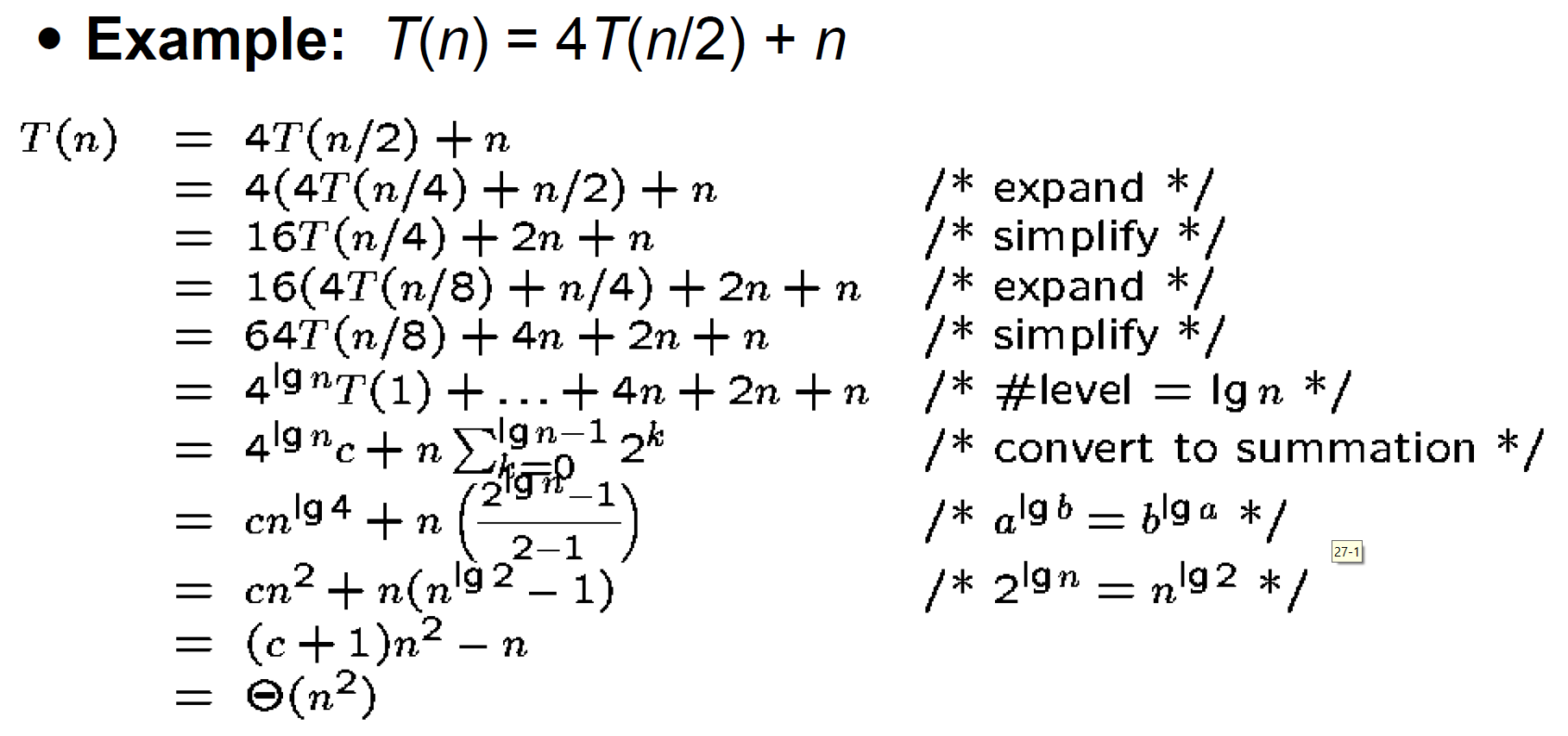
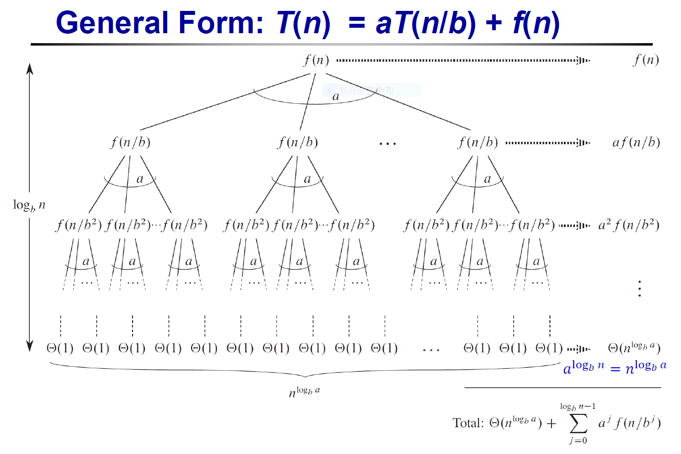
unrolling
- iteration
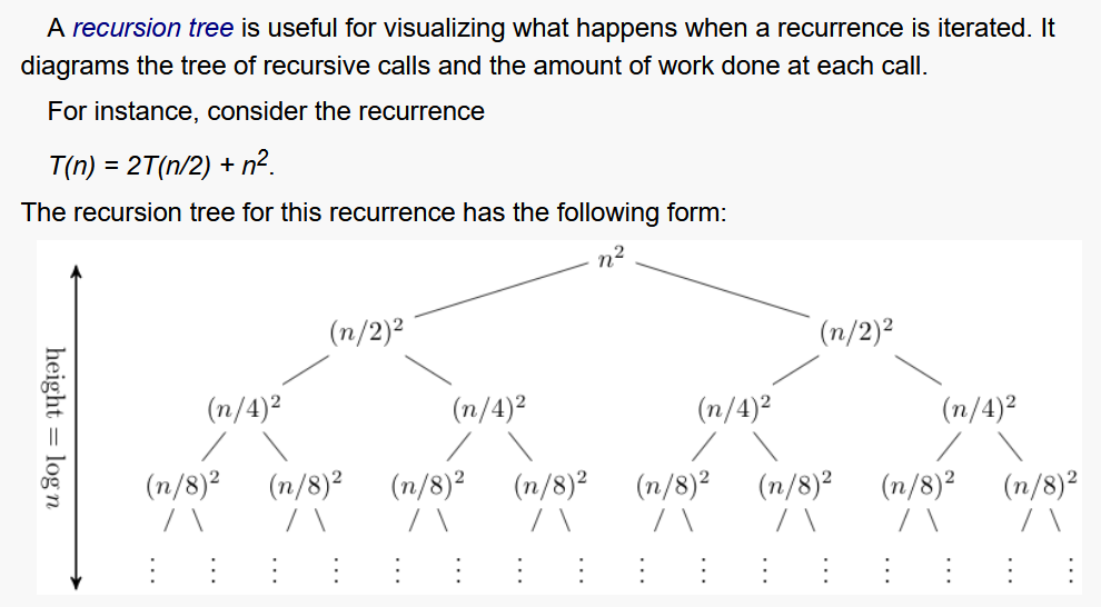
- recursion tree
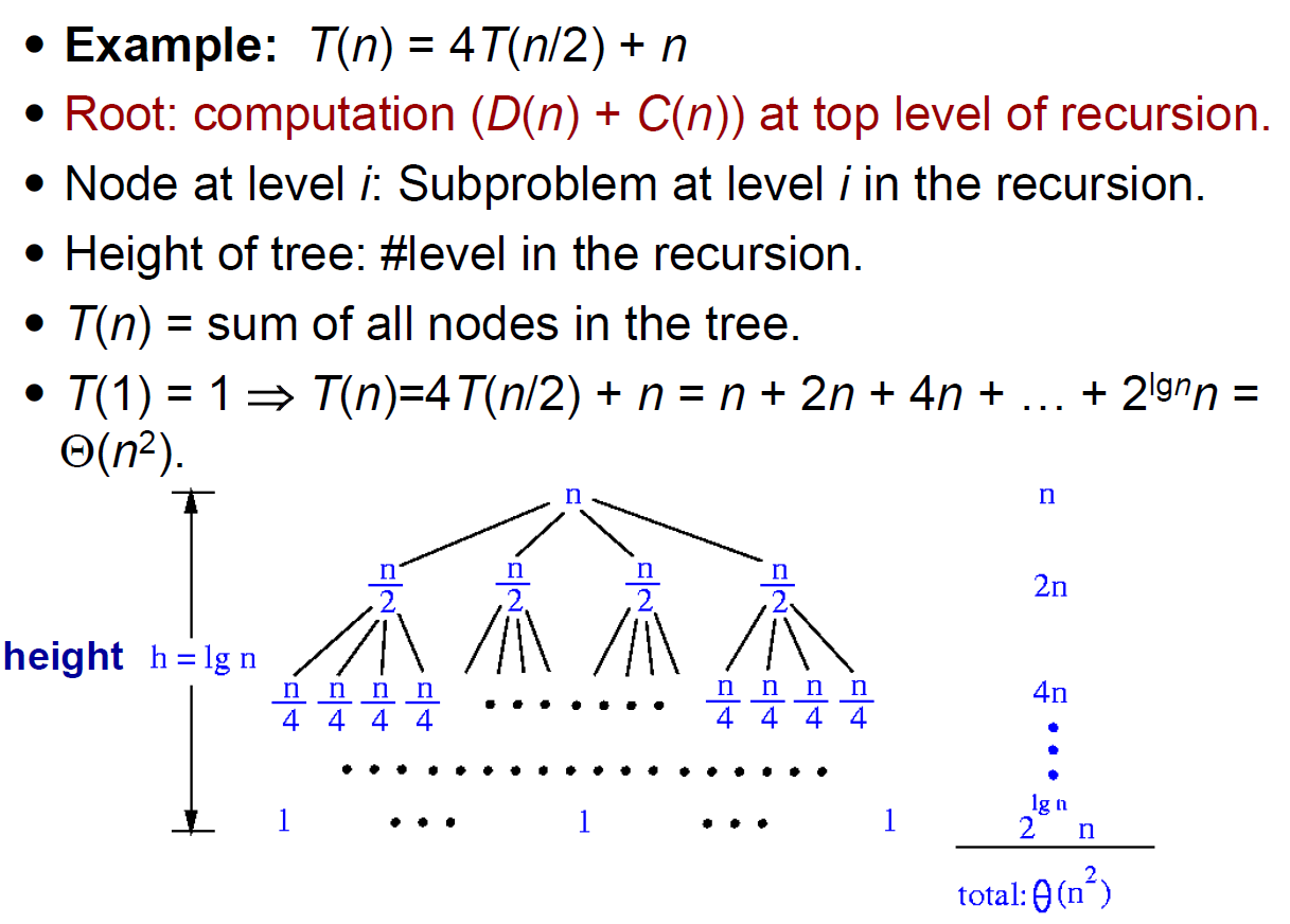
- do n work and call n/2 4 times at level n
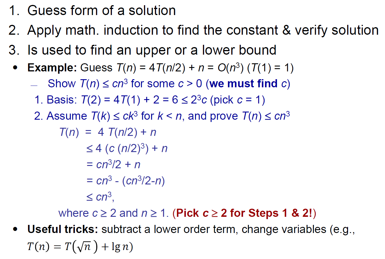
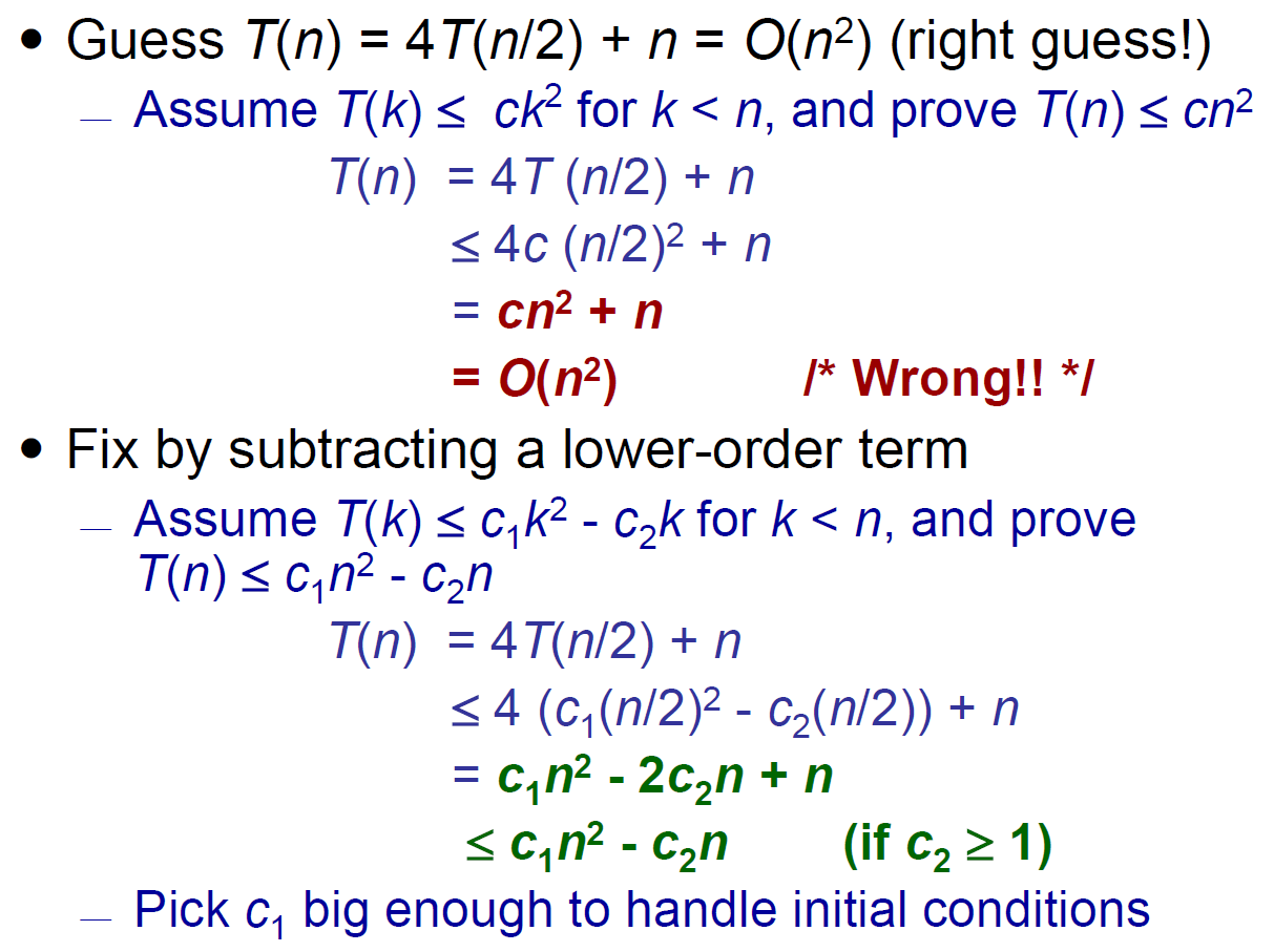
substitution
- guess and proof (with strong induction)
- 不太需要管 n/2 是不是整數之類的的問題
- 猜答案方法
- 隨便畫個 recursion tree
- e.g.
- strong induction
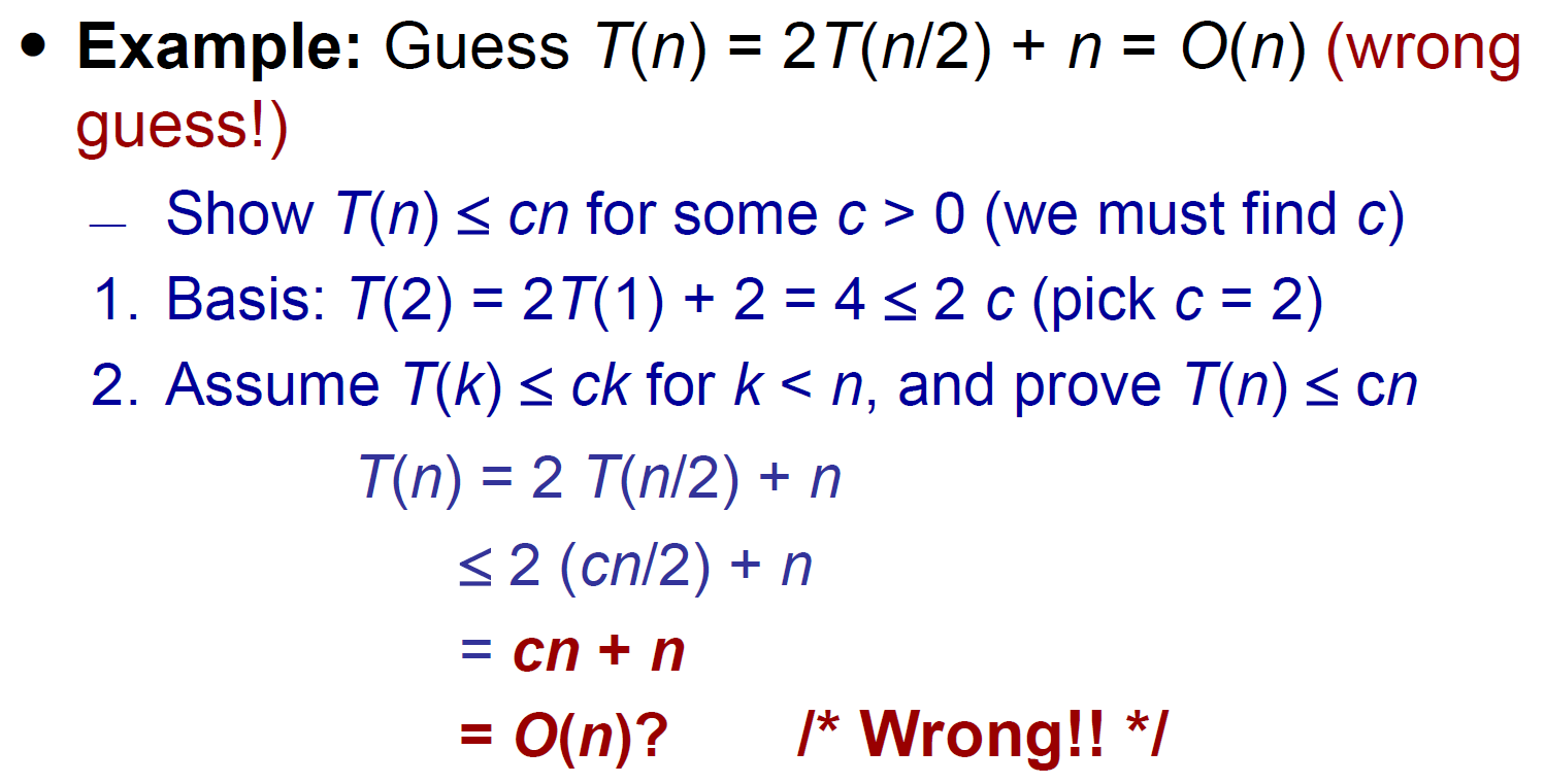
- >cn → wrong
- 減掉一個 lower order term
- 考法
- 跟你說要證什麼 (不用猜)
Master theorem
- Data Structure#Master Theorem
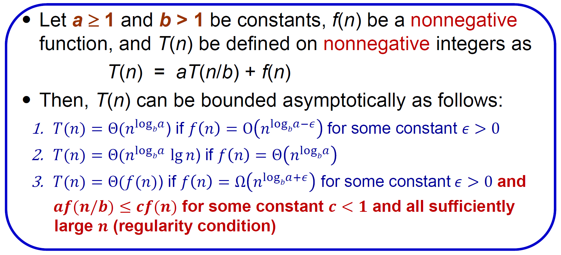
- 最下層最好用 k or c 代替,之後再 asymptotic
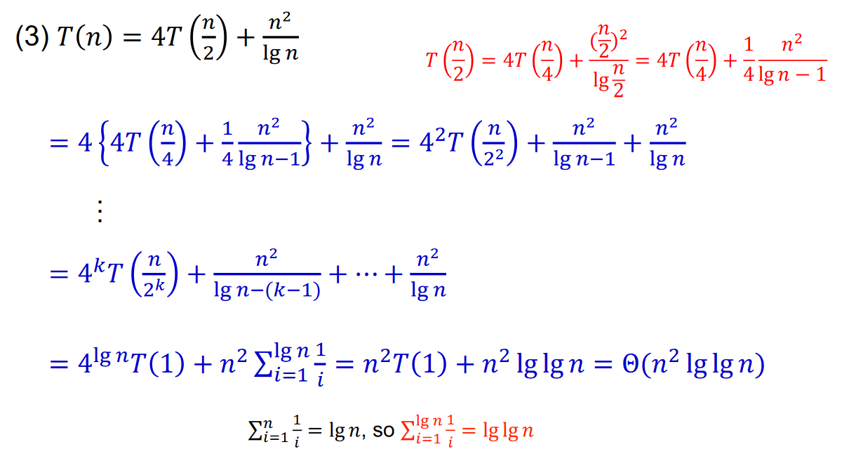
examples
- \(T(n)=T(n/2)+T(n/4)+n\in\Theta(n)\)
- substitution
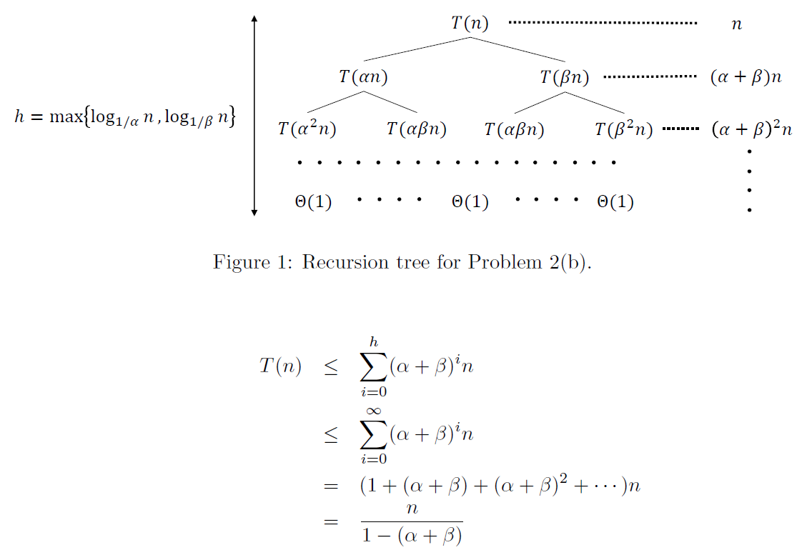
- 最後分母是 1-(p+q)
- if p+q>1 && p,q>1
- \(2^{log_{1/q} (n)} <= leaves <= 2^{log_{1/p} (n)}\)
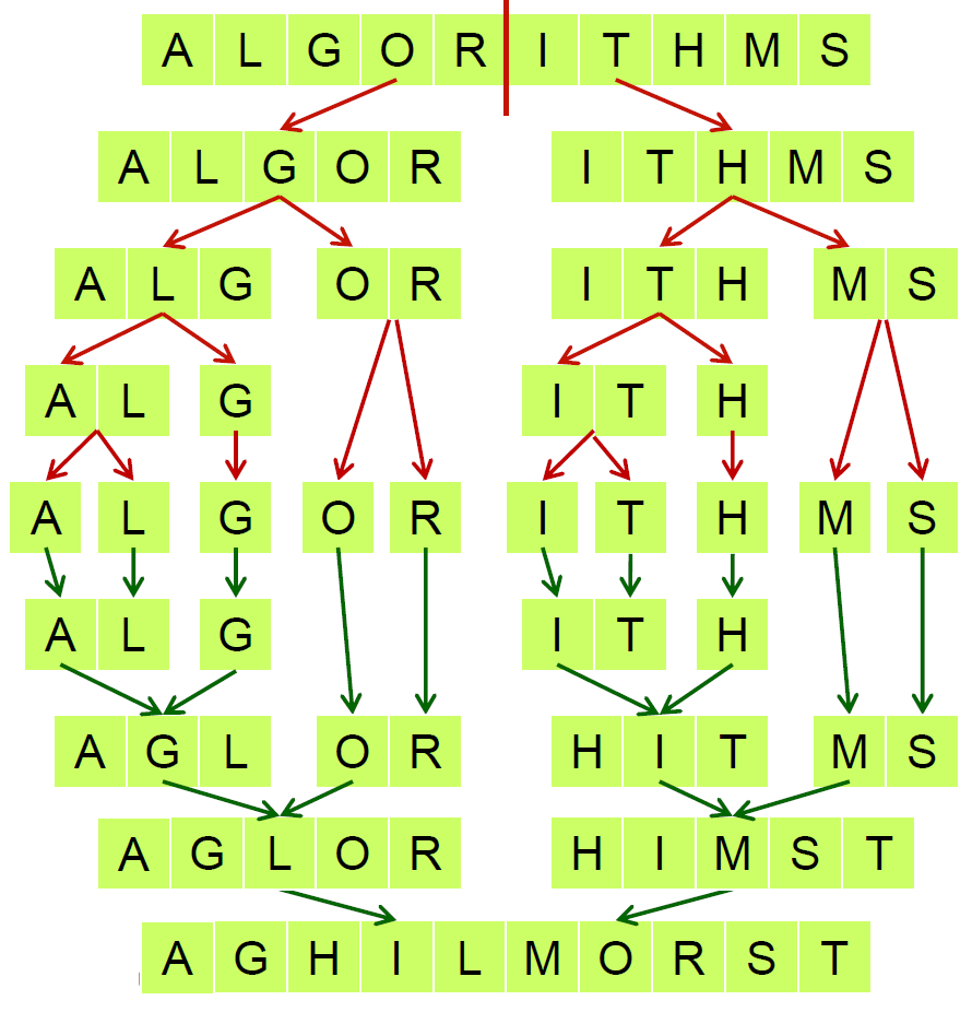
merge sort
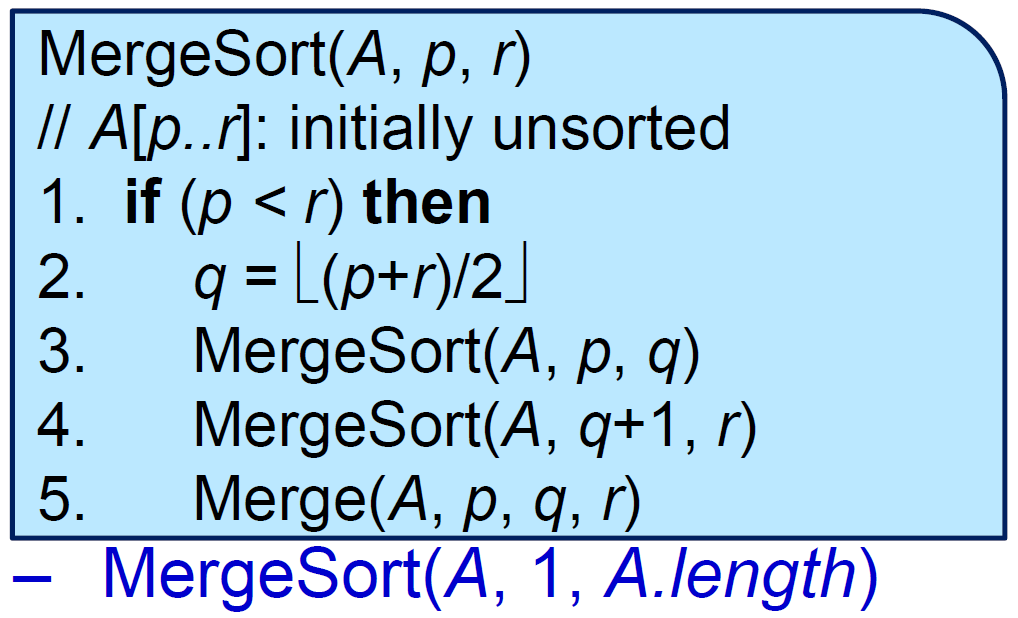
MergeSort(A,p,r) //T(n)
    if (p<r) then //1
        q=Math.floor((p+r)/2) //1
        MergeSort(A,p,q) //T(n/2)
        MergeSort(A,q+1,r) //T(n/2)
        Merge(A,p,q,r) //n

MergeSort(A,1,A.length)
 -
- Merge()
- \(\in \Theta(n)\)
- 兩個已經 sort 好的 n/2 array,做 sorting → n 次比較
- 需要額外 memory
- 兩半各一個 auxiliary array
- pseudo code
-  -
- 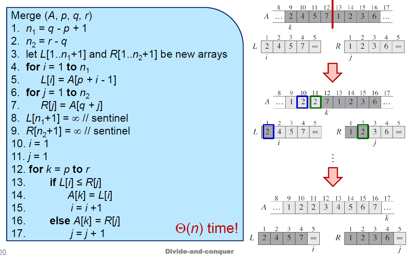 - 4-5: L = 左半 array
- 6-7: R = 右半 array
- 8-9: L & R 的最後一項設成無限
- 10-17: 從小到大,一個一個比對 L & R,較小者填進 main array
- time complexity \(\in \Theta(nlgn)\)
-
- 4-5: L = 左半 array
- 6-7: R = 右半 array
- 8-9: L & R 的最後一項設成無限
- 10-17: 從小到大,一個一個比對 L & R,較小者填進 main array
- time complexity \(\in \Theta(nlgn)\)
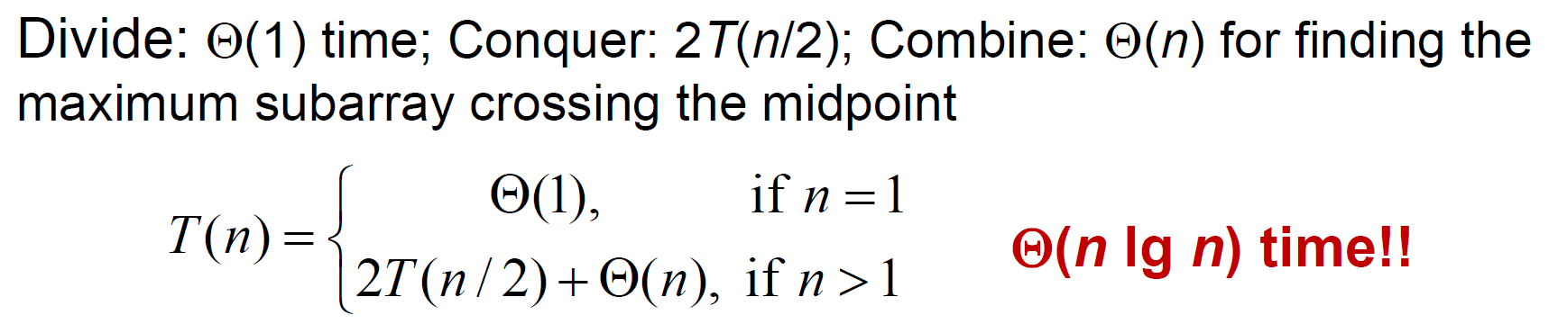
- 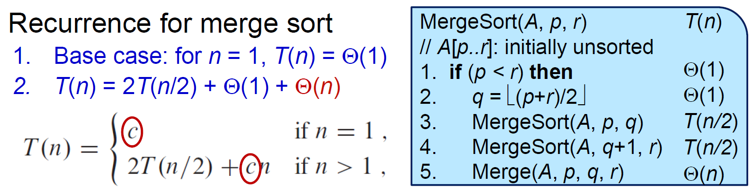 - 其實是 \(T(n)=T(\lfloor n/2\rfloor)+T(\lceil n/2\rceil)+cn\) \(\because\)左右數量非 n/2,但可忽略
- using unrolling - recursion tree
-
- 其實是 \(T(n)=T(\lfloor n/2\rfloor)+T(\lceil n/2\rceil)+cn\) \(\because\)左右數量非 n/2,但可忽略
- using unrolling - recursion tree
- 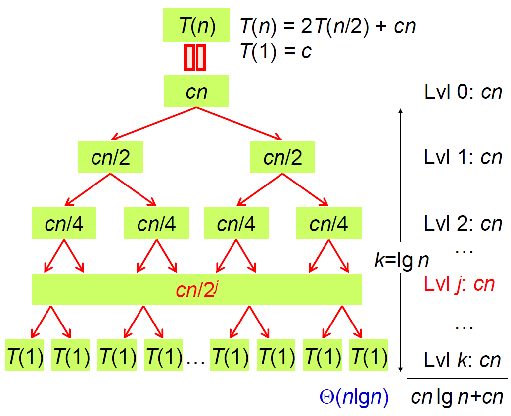 - \(cn(lgn+1)\)
- using substitution
- 猜 \(O(nlgn)\)
- basis & inductive
- beats #insertion sort
- properties
- stable
- not in-place
- \(cn(lgn+1)\)
- using substitution
- 猜 \(O(nlgn)\)
- basis & inductive
- beats #insertion sort
- properties
- stable
- not in-place
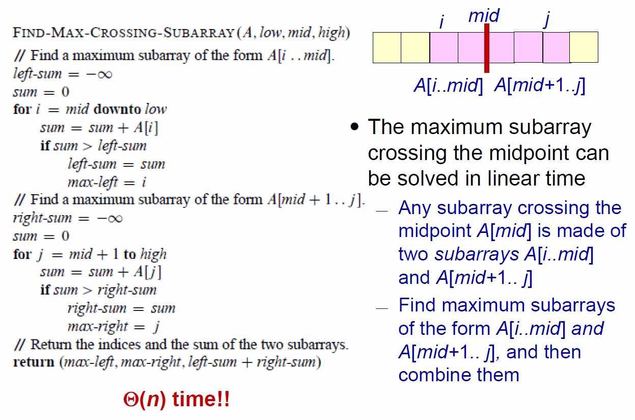
maximum subarray
- leetcode maximum subarray 四部曲
- 分成左&右&橫跨部分
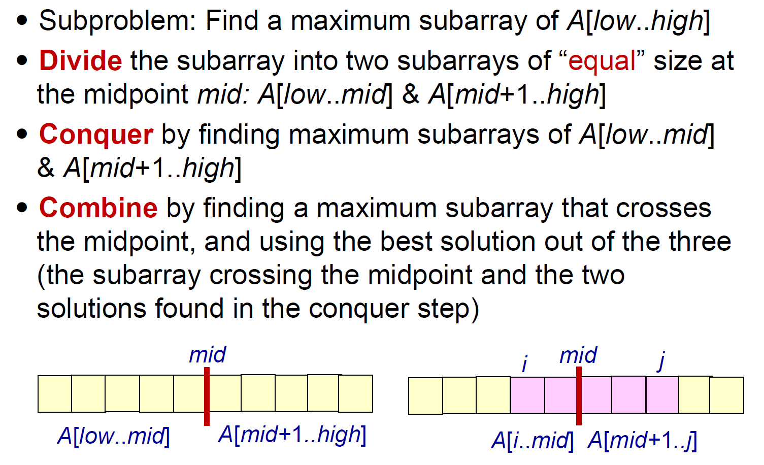
- 橫跨部分
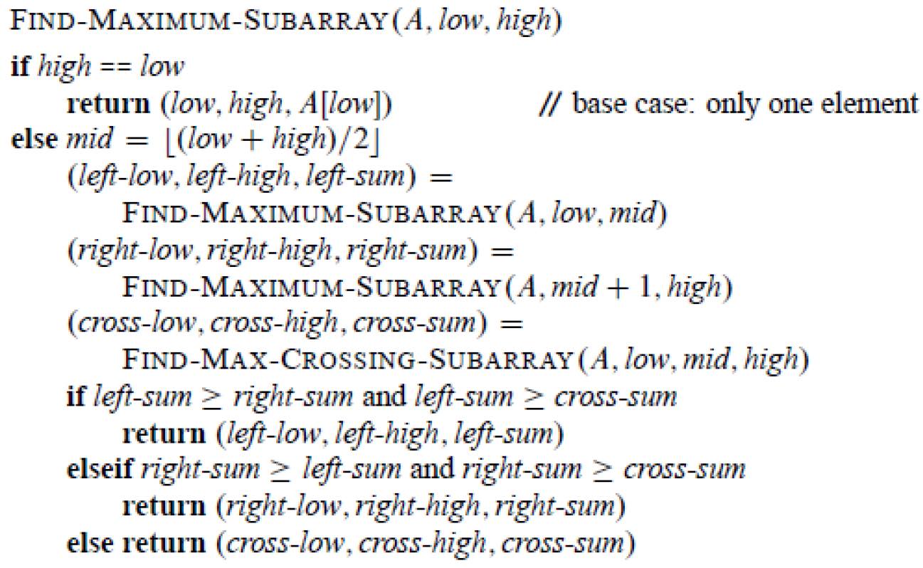
- \(\Theta(nlgn)\)
Strassen's method
matrix multiplication
- normal \(\in O(n^3)\)
- \(n^2\) elements, each is the sum of \(n\) values
- divide into 4 n/2xn/2
- \(\in \Theta(n^{lg8})=\Theta(n^3)\)
- 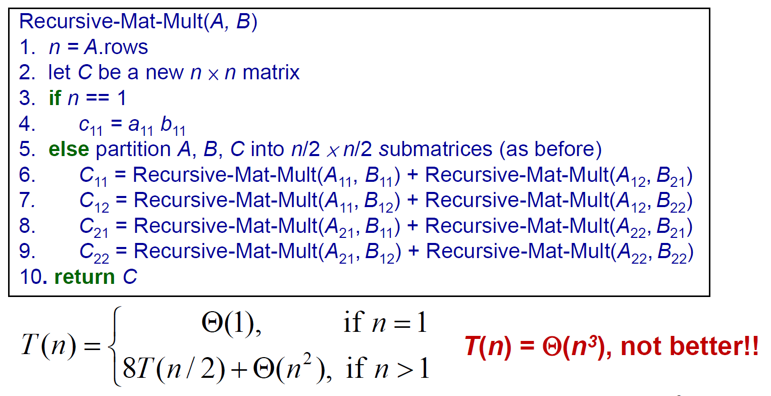 - Master theorem
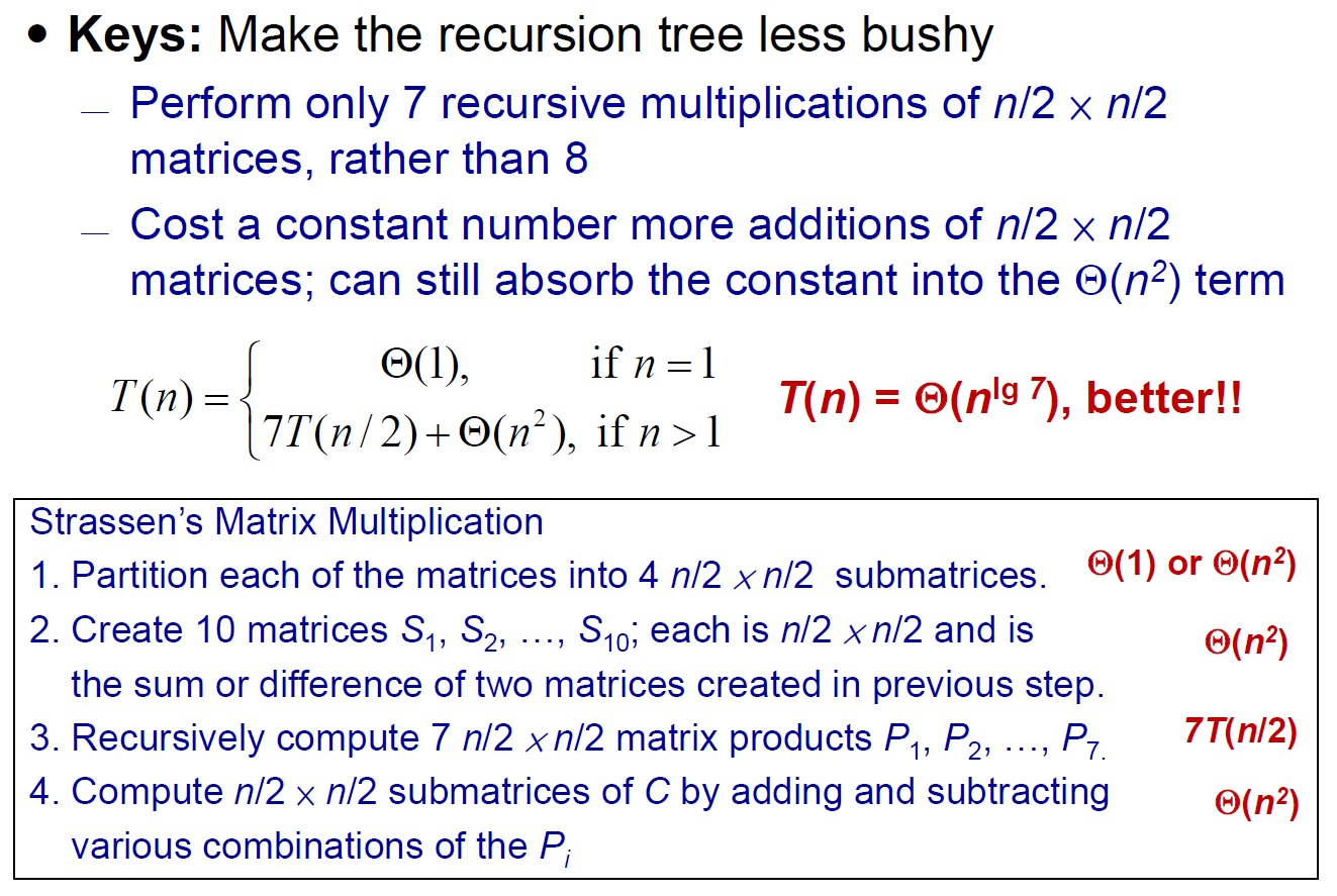
- 只要 T(n/2) 係數是 7,就會 \(\in o(n^3)\)
- Strassen's method \(\in \Theta(n^{lg7}) \in o(n^3)\)
-
- Master theorem
- 只要 T(n/2) 係數是 7,就會 \(\in o(n^3)\)
- Strassen's method \(\in \Theta(n^{lg7}) \in o(n^3)\)
- 
Sorting
sorting comparisons
- time complexity
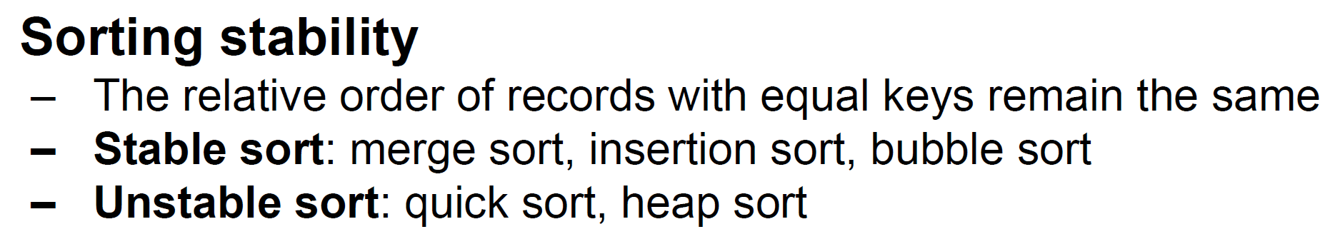
- stable
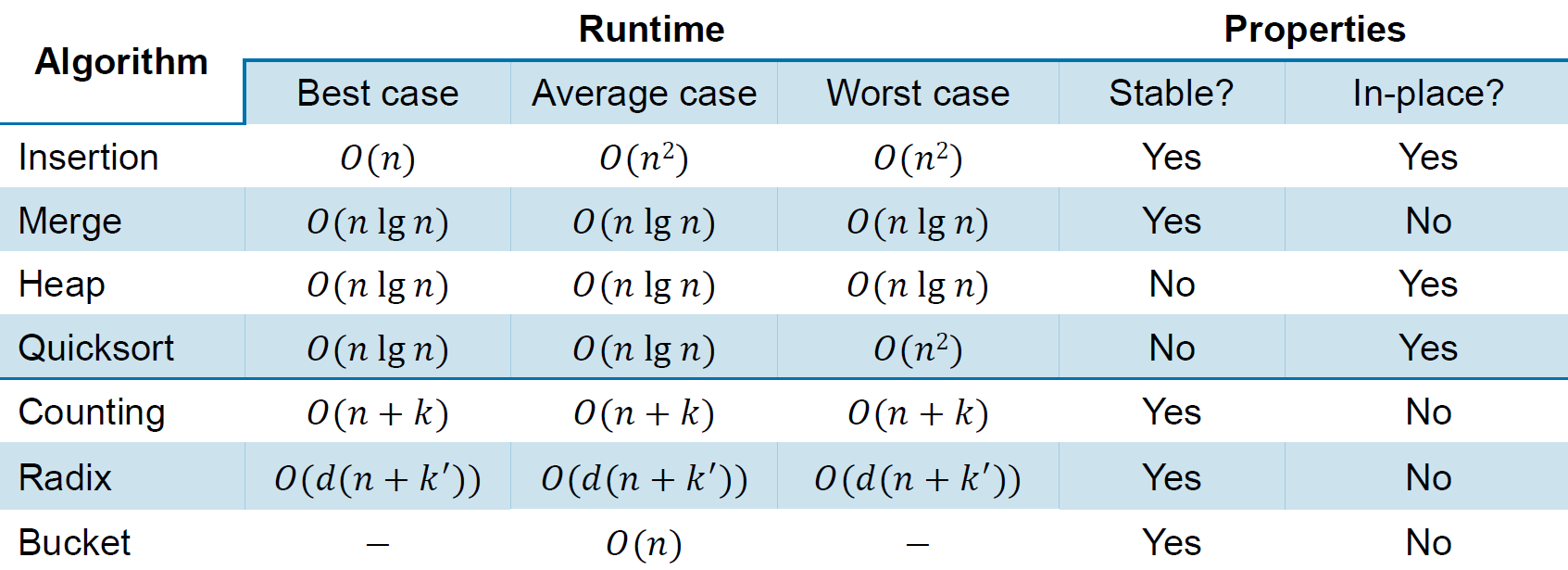
insertion sort
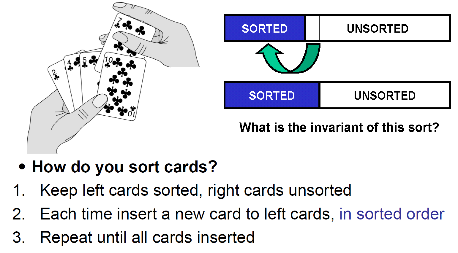
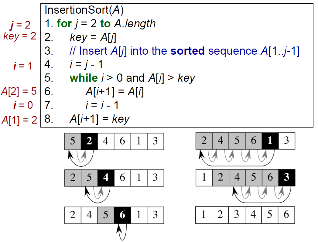
void insertion_sort(int x[],int length)//define function
{
  int key,i;
  for(int j=1;j<length;j++)
  {
     key=x[j];
     i=j-1;
     while(x[i]>key && i>=0)
     {
         x[i+1]=x[i];
         i--;
     }
     x[i+1]=key;
  }
}
Quicksort
- use divide-and-conquer
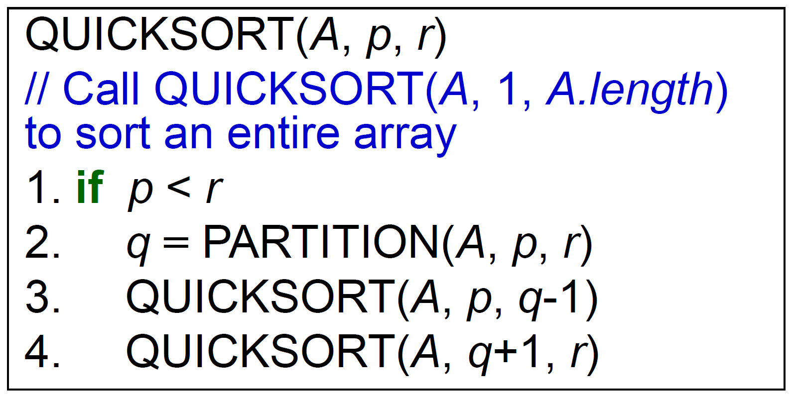
- partition 後基準的位置的左右再各執行
- partition
- 選基準點 (e.g. rightmost)
- 掃過 array,把小於基準的放在前面,大於基準的放在後面,最後基準放前後之間
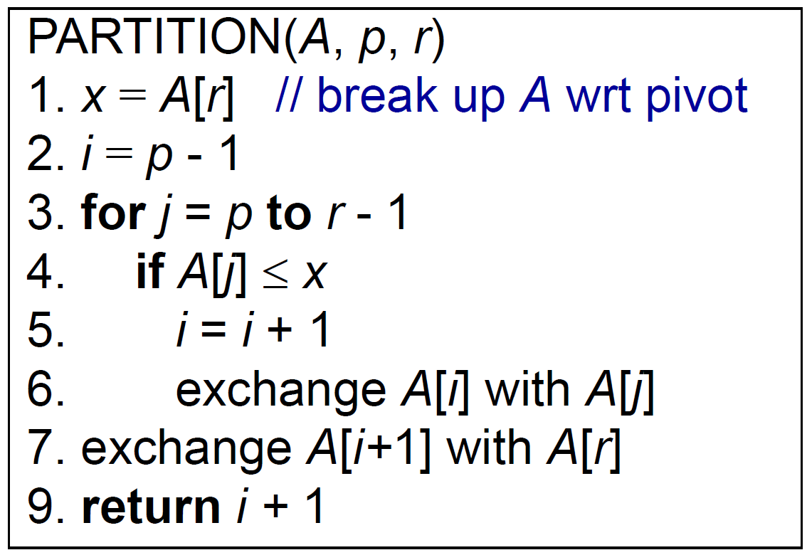
- return 最後基準點在的位置
- \(\Delta i=\) 小於基準者的數目
- return 最後基準點在的位置
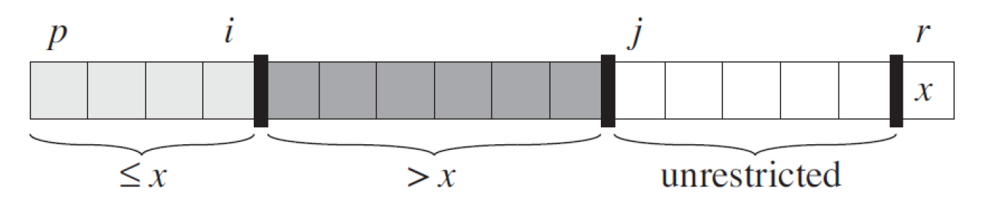
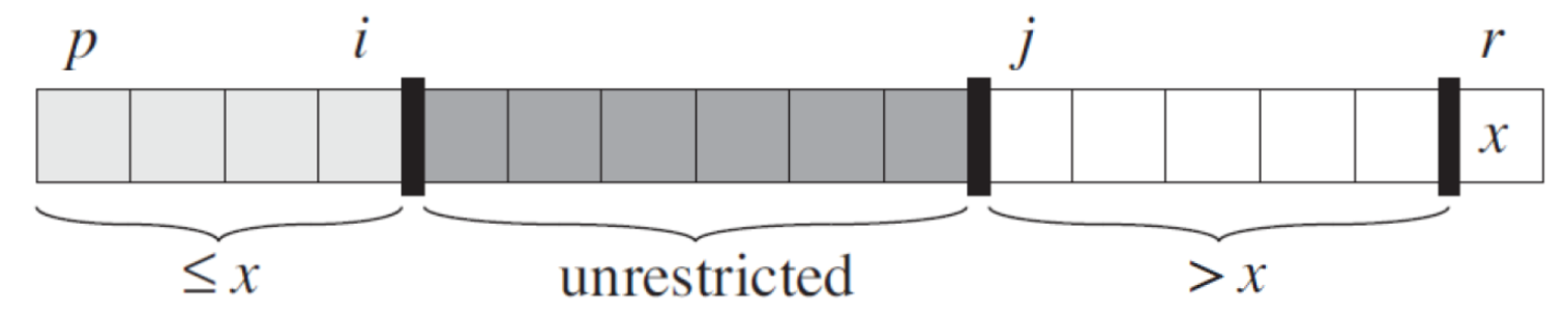
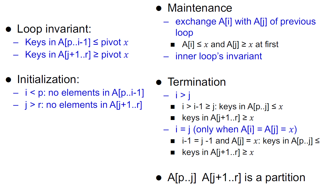
- loop invariant
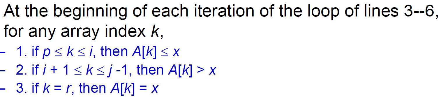
- unrestricted: 還沒掃到的
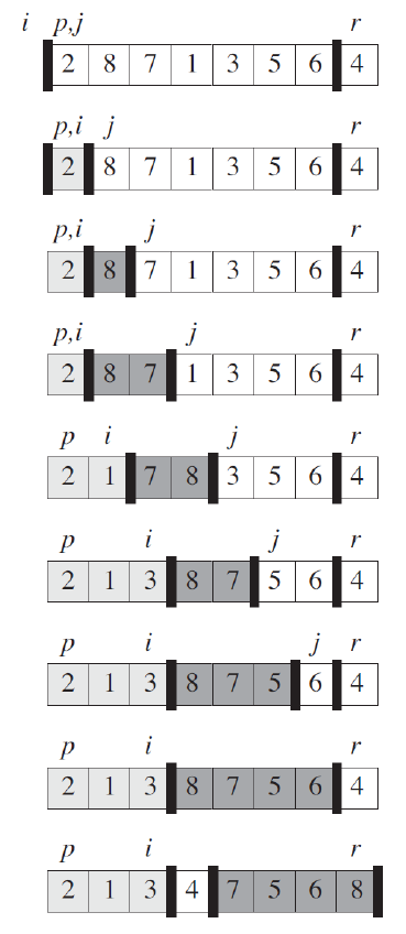
- 用 swap 的
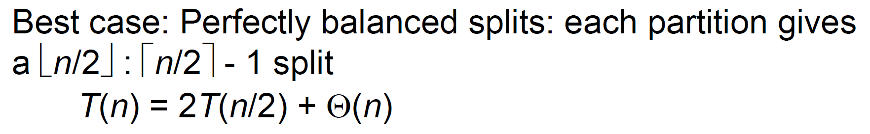
- time complexity
- best case \(\in\Theta(nlgn)\)
- 每個都均勻分
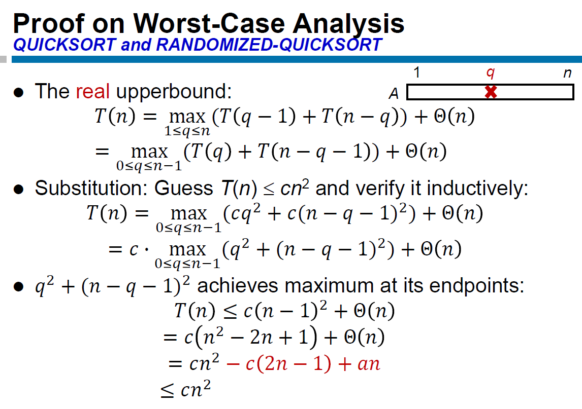
- worst case \(\in\Theta(n^2)\)
- sorted OR reversely sorted
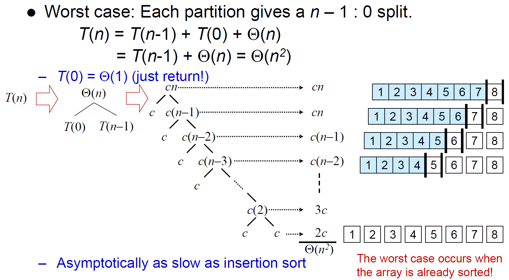
- practically very good, but asymptotically bad
- best case \(\in\Theta(nlgn)\)
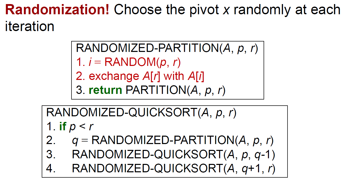
randomized partition
- random 選一個 element 跟最後一位交換
- time complexity
- worst case
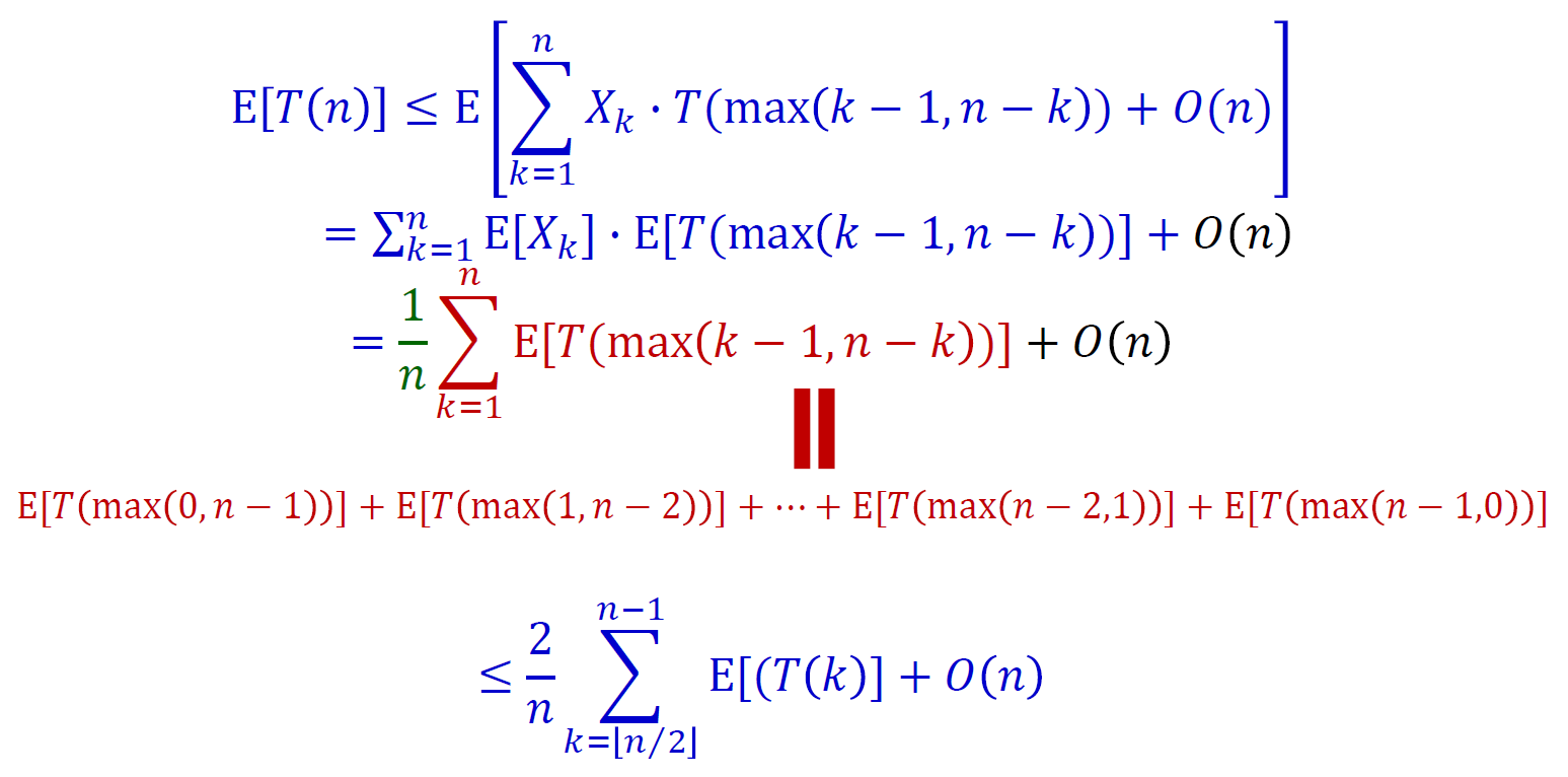
- expected \(\in O(nlgn)\)
- method 1
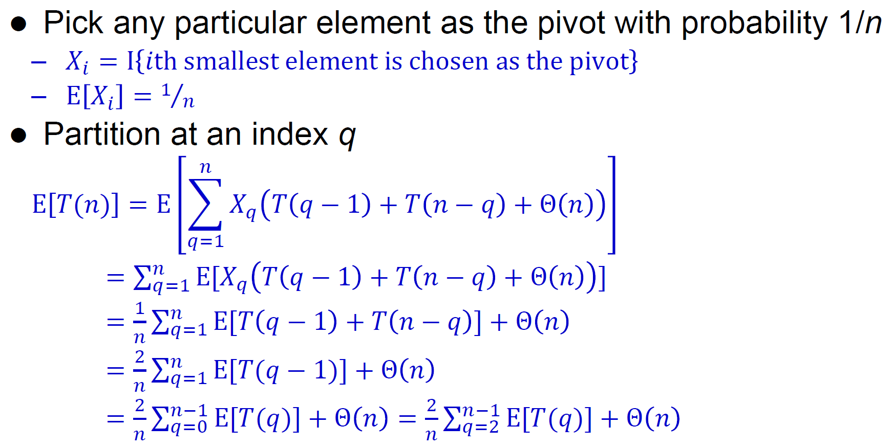
- \(X_q=1/n\)
- sum(T(q-1))=sum(T(n-q))
- 忽略 q=0, 1
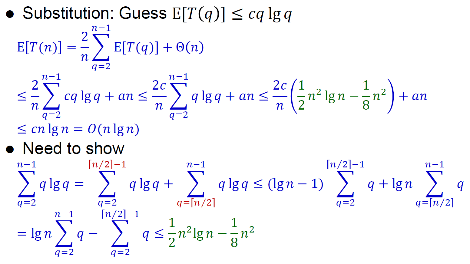
- 猜 nlgn
- method 2
- runtime \(\in O(n+X)\)
- n elements → max n partitions
- X comparisons
- 只有 pivot 需要跟別人比較
- 兩 elements 至多比較一次
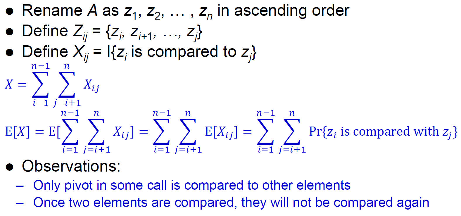
- E[X] = expected X
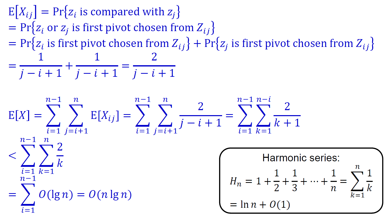
- \(E[X_{ij}] = z_i\) or \(z_j\) 為 pivot 的機率
- method 1
- worst case
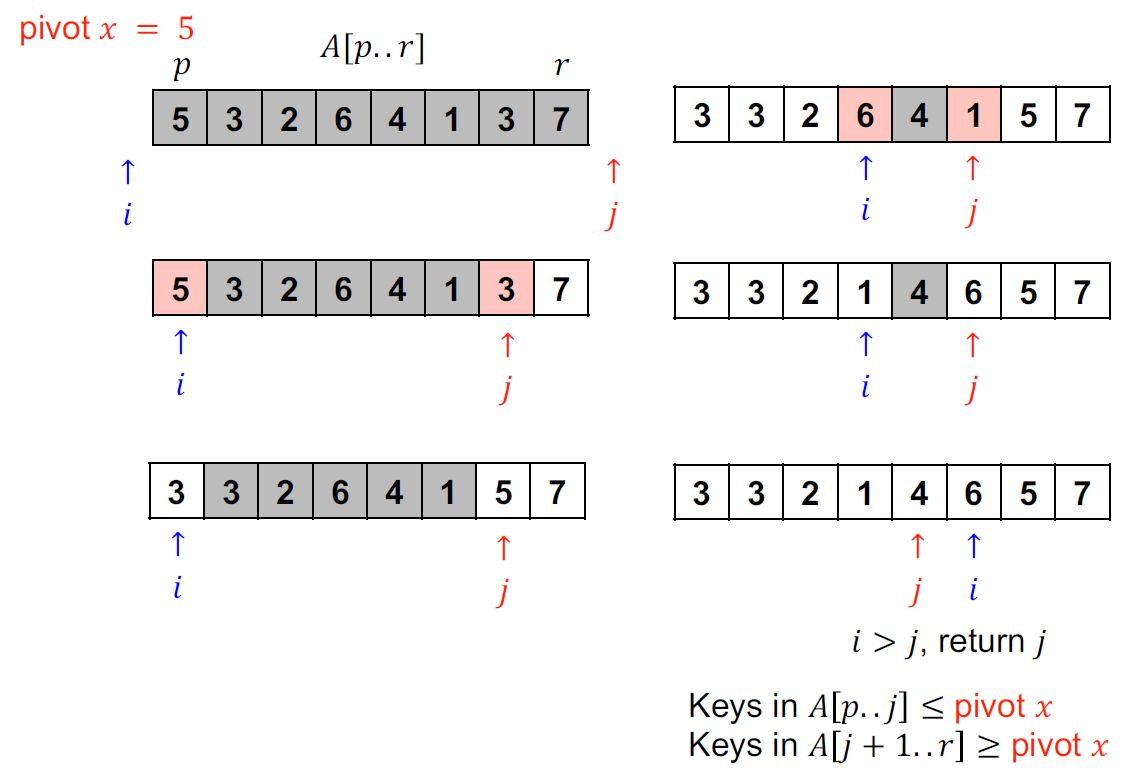
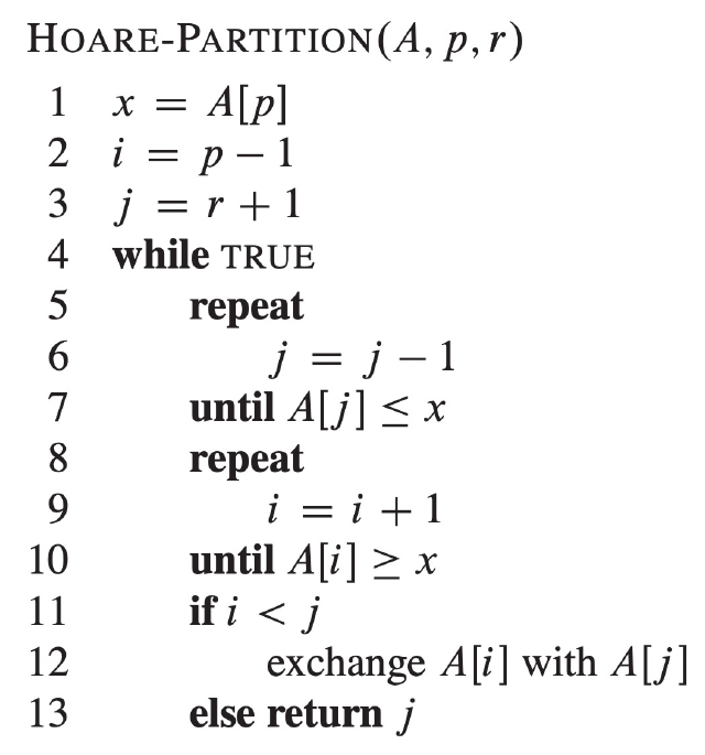
Hoarse partition
- 原始提出版本
- ==很愛考==
- i & j 交疊 → 完成
- pseudo code
- loop invariant
- 好處壞處 complexity 都跟課本版本一樣
heapsort
heap (priority queue)
- Data Structure#bineary heap
- heapify
- percolate down
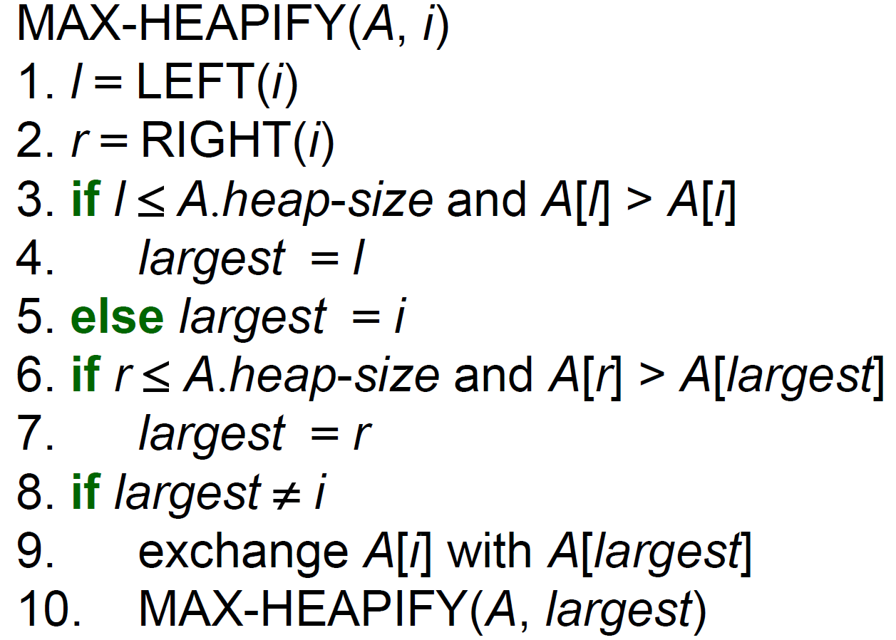
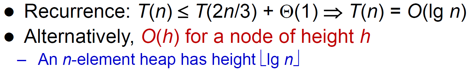
- worst case
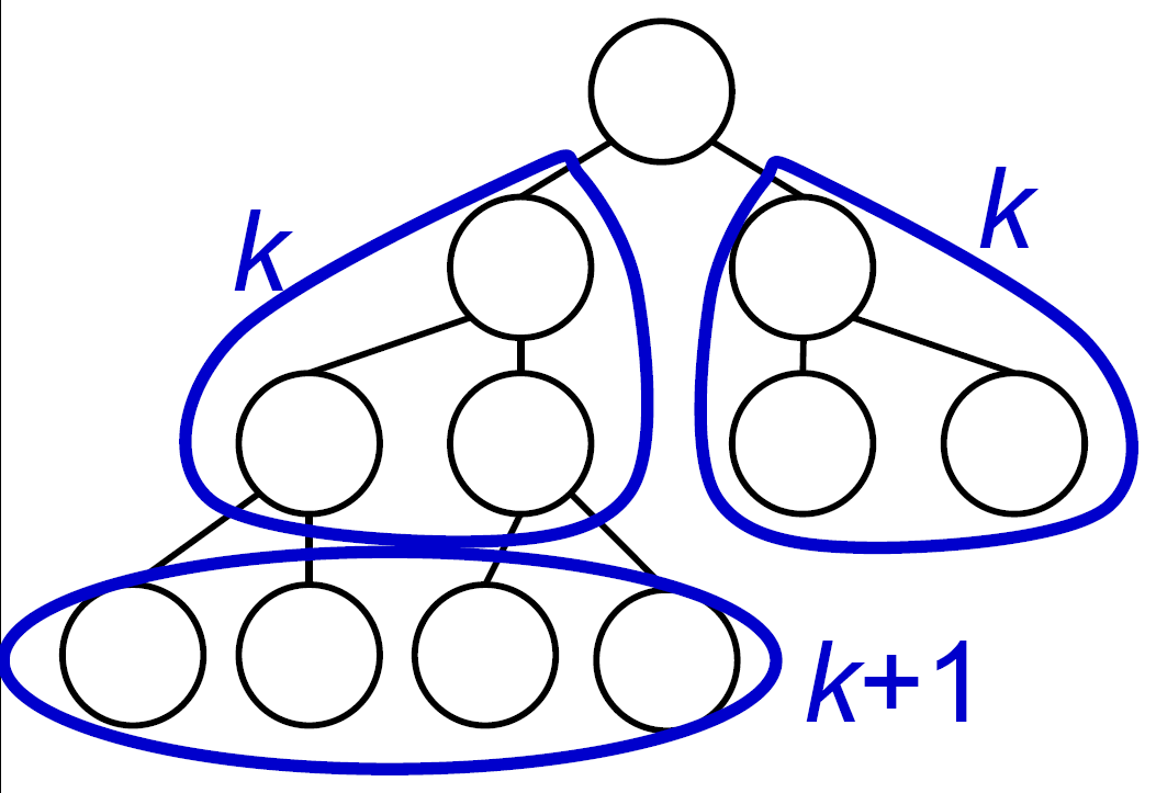
- 最下層 half full → 左邊 size <= 2n/3
- time complexity
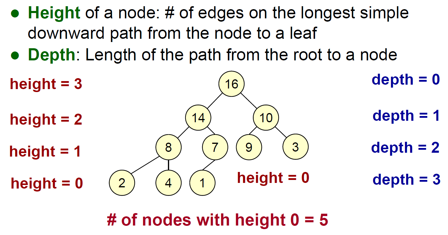
- depth vs. height
- binary tree to max-heap
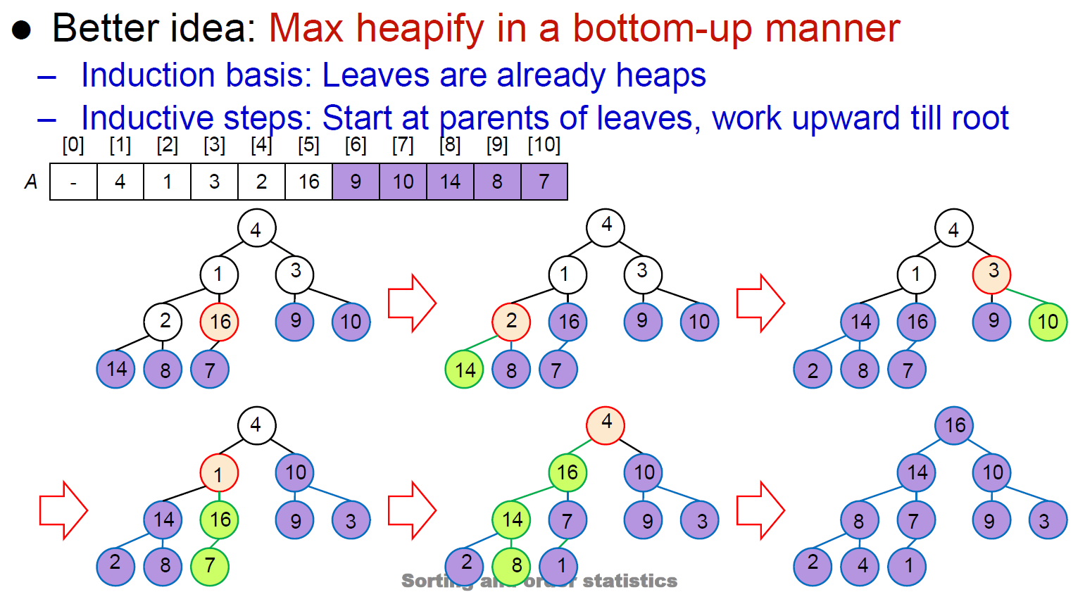
- bottom-up, percolate up
- build max heap \(\in O(n)\)
- bottom-up heapify
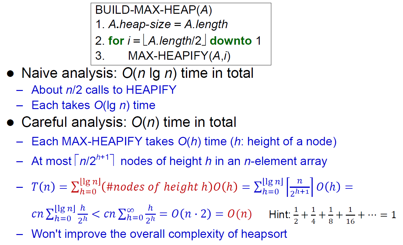
- taylor series
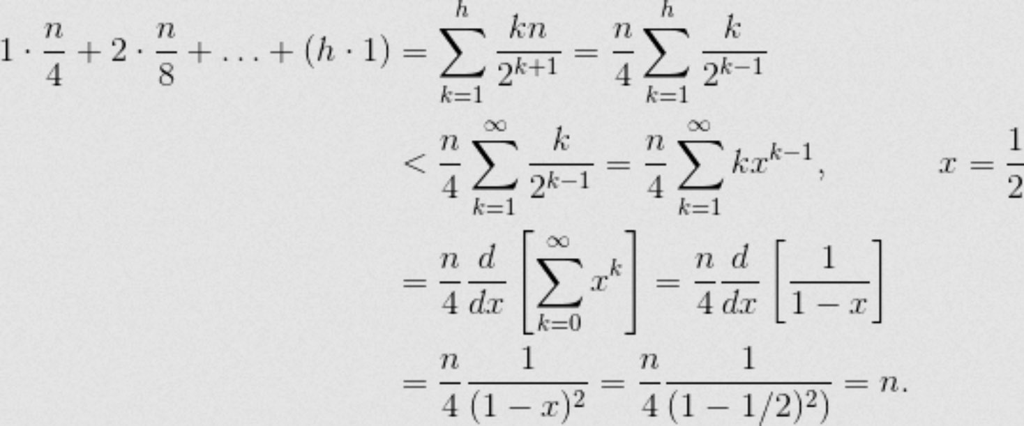
- https://stackoverflow.com/a/18742428/15493213
heapsort
- 用 max-heap 做 selection sort
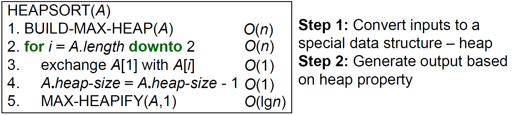
- 存成 max-heap → 重複把 delete min i.e. 把 max (第一項) 跟 bottom-level 最右 (第二項) 交換 → 成功排序
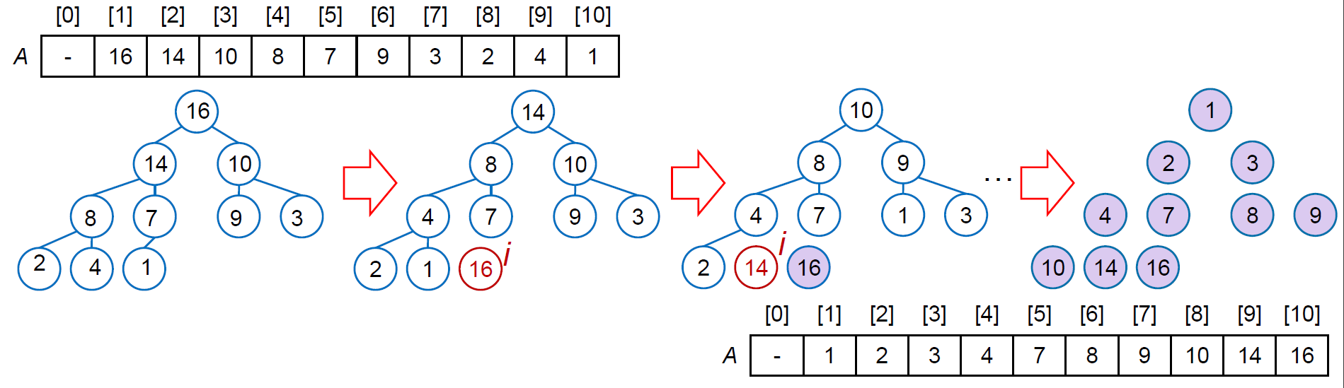
- time complexity \(\in O(nlgn)\)
- heapify O(lgn)
- iterate n 次
- in-place
- 都在原本的 array 上面做
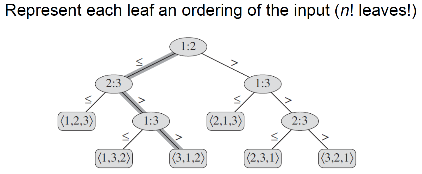
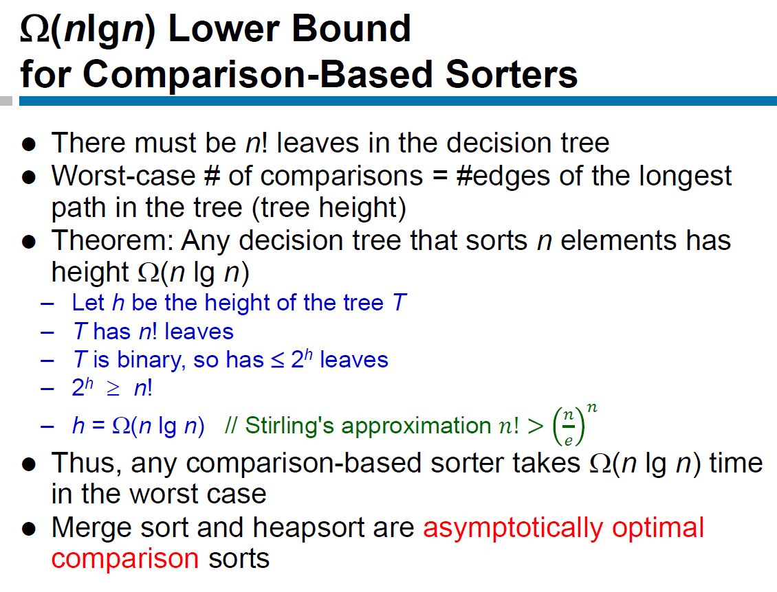
comparison-based sorters
- decision tree
- leaf 代表 n 個數字排序可能的結果 → n! leaves
sorting in linear time
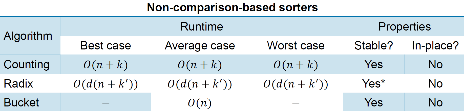
 radix & bucket sort use other sorters to do the actual sorting
counting sort
- 有 m 個數字 <= k → 把 k 放在位置 m
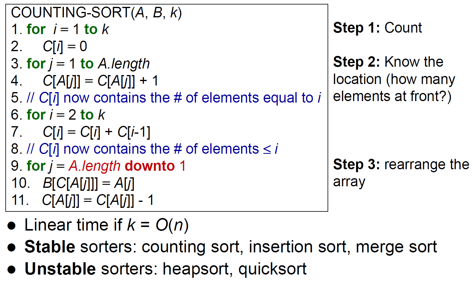
- stable
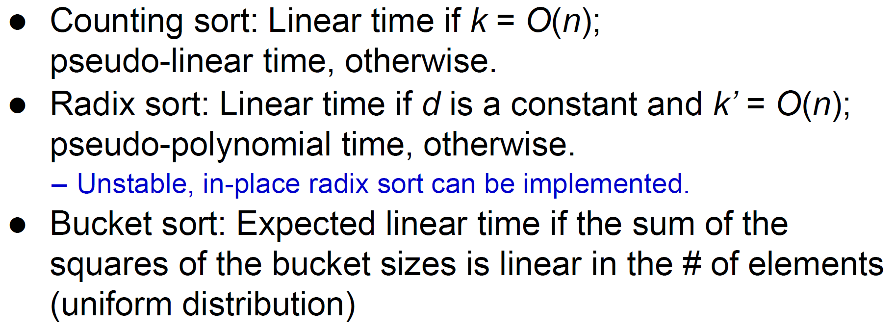
- time complexity \(\in O(n+k)\)
- \(\in O(n)\) if \(k\in O(n)\)
- pseudo-linear time otherwise
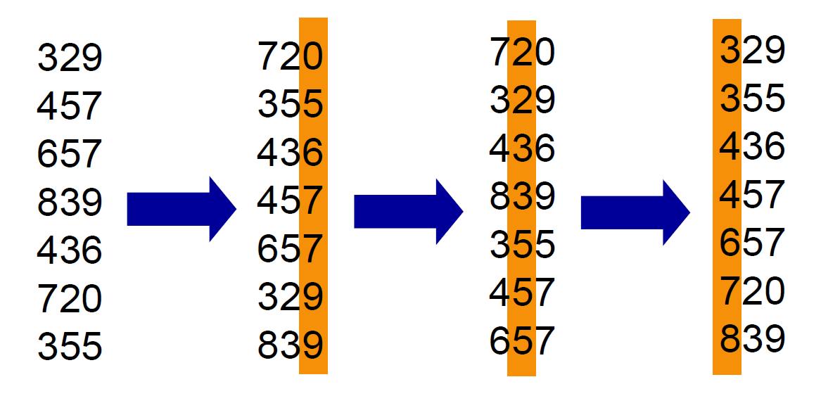
radix sort
- 一個位數一個位數 sort,從最小位數開始
- 需 stable sorter
- counting sort
- not in-place → need more memory
- insertion sort
- fast when size small
- counting sort
- time complexity \(\in O(d(n+k))\)
- n d-digit numbers
- each digit has k possible values
- \(\in O(n)\) if \(d\in O(1)\) & \(k\in O(n)\)
- 如果用 \(O(nlgn)\) sorter 就是 \(O(dnlgn)\)
- stable, in-place or not depends on what sorter used (to sort each digit)
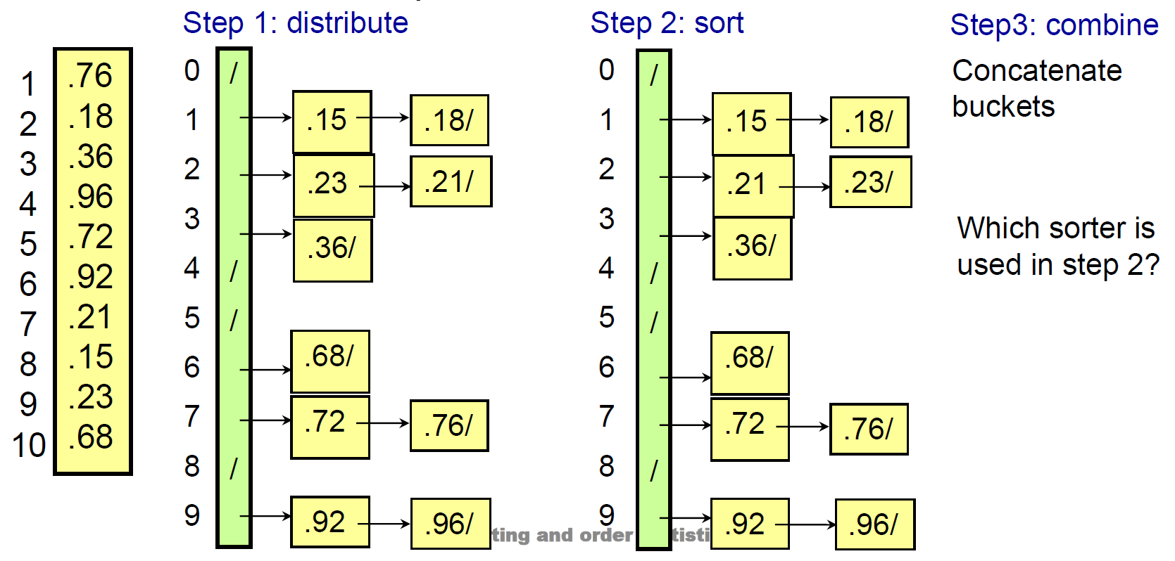
bucket sort
- 分成很多個同樣區間的 bucket,先把各數字放進各自的 bucket,在各 bucket 裡 sort,最後 combine
- k buckets
- 區間為 1 → #counting sort
- space complexity \(\in O(n+k)\)
- time complexity
- iterate all elements, in each bucket, but will iterate n elements at most
- expected & best case \(\in O(n+k)\)
- worst case \(\in O(n^2)\)
- when all elements go to 1 bucket → runtime depends on what sorter used → worst case \(\in O(n^2)\)
order statistics
ith order statistic = ith smallest element
selection
- pseudo code
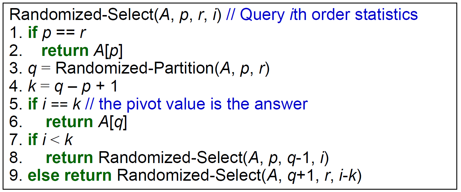
- q = random 找的這個 element 排序後排在的位置
- time complexity

- expected linear time
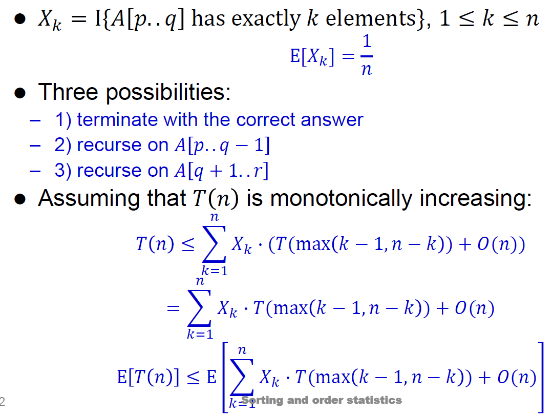
- 猜 linear time
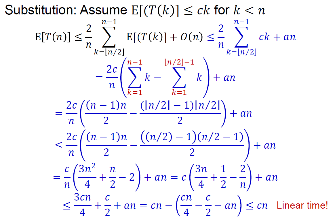
- worst case linear time
- 五五一組,找到各組 median,再找這些 median 的 median
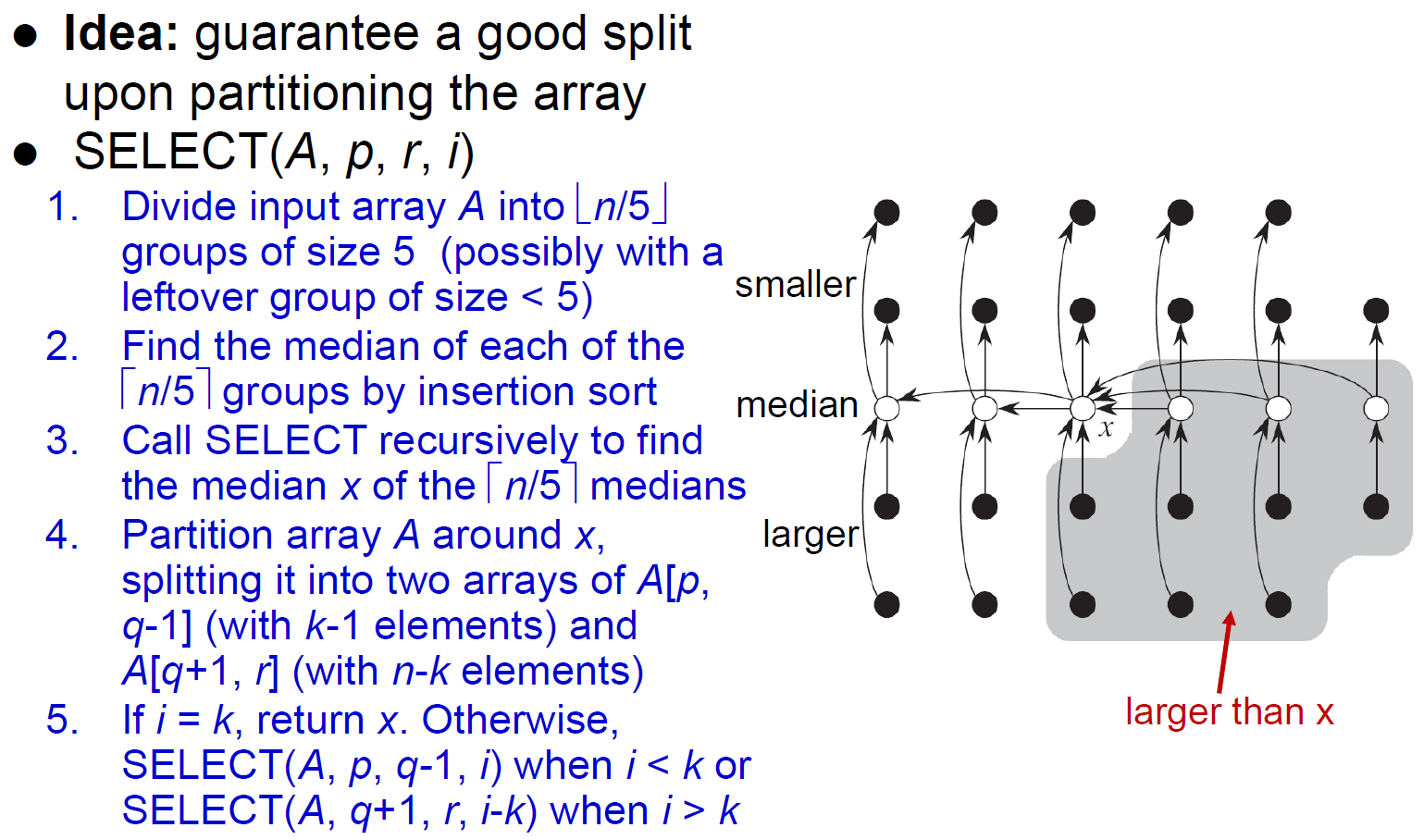
- 可用這個 procedure 去幫 #Quicksort 找 median → guarantee O(nlogn)
Trees
Binary Tree
- see Data Structure#Binary Tree
- tree construction
- worst case \(O(n^2)\)
- average case \(O(nlgn)\)
- height
- worst case \(h\in O(n)\)
- skewed
- best case \(h\in O(lgn)\)
- balanced
- worst case \(h\in O(n)\)
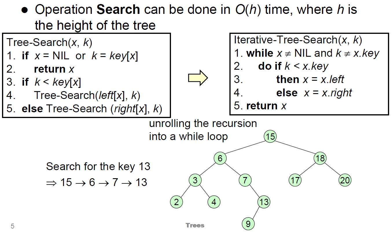
- most operations \(O(h)\)
operations
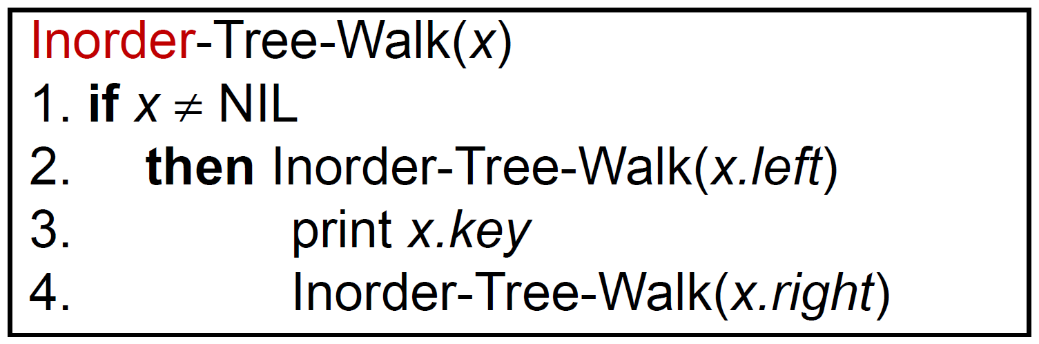
- traversal
- inorder/infix
- preorder/prefix
- postorder/postfix
- inorder/infix
- search
- successor
- 比我大的最小的 node
- 有 right subtree → right subtree 的 min
- 沒 right subtree → 找我是誰的 predecessor
- irl operation: 往左上走直到轉折 as in line 3-6
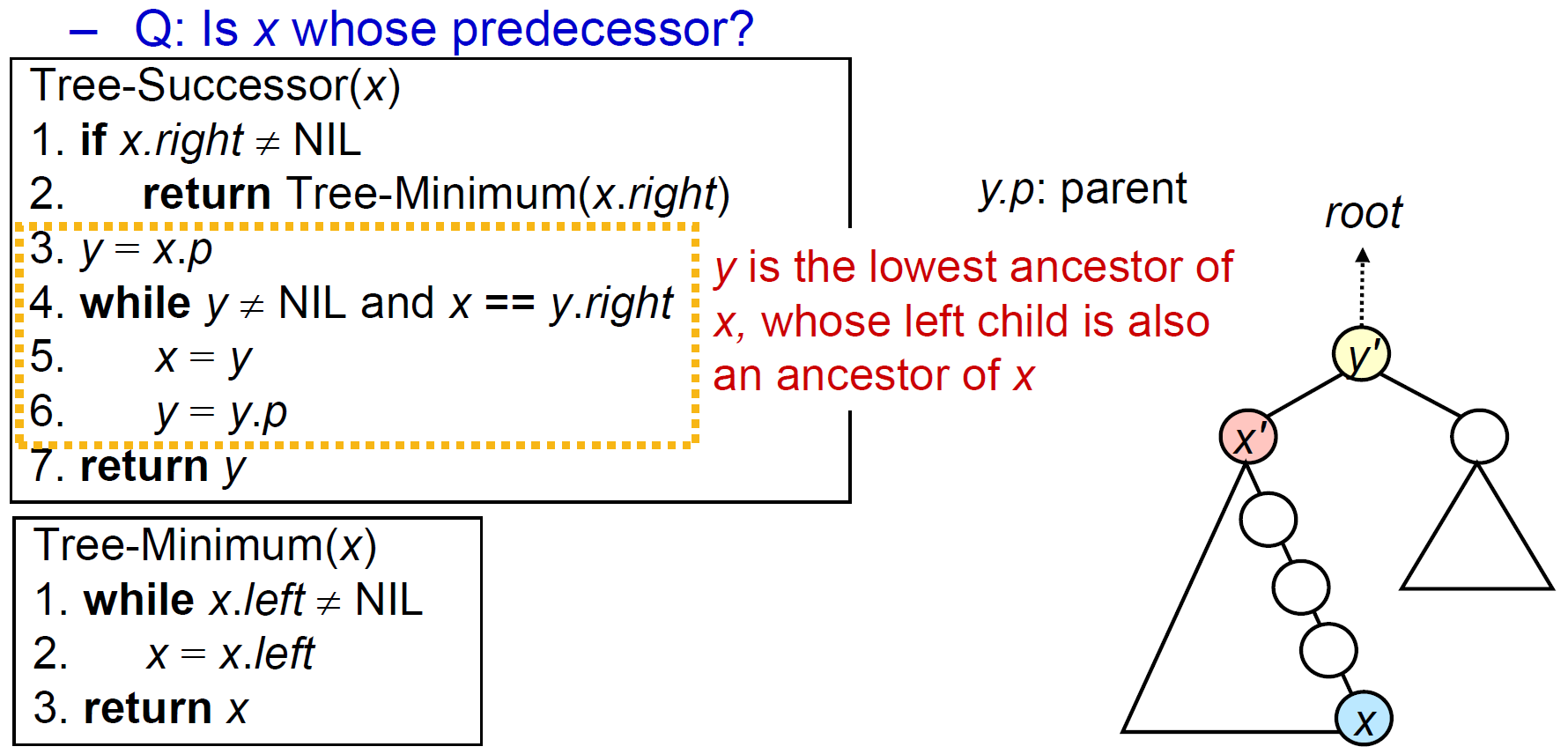
- 比我大的最小的 node
- predecessor
- 比我小的最大的 node
- 有 left subtree → left subtree 的 max
- 比我小的最大的 node
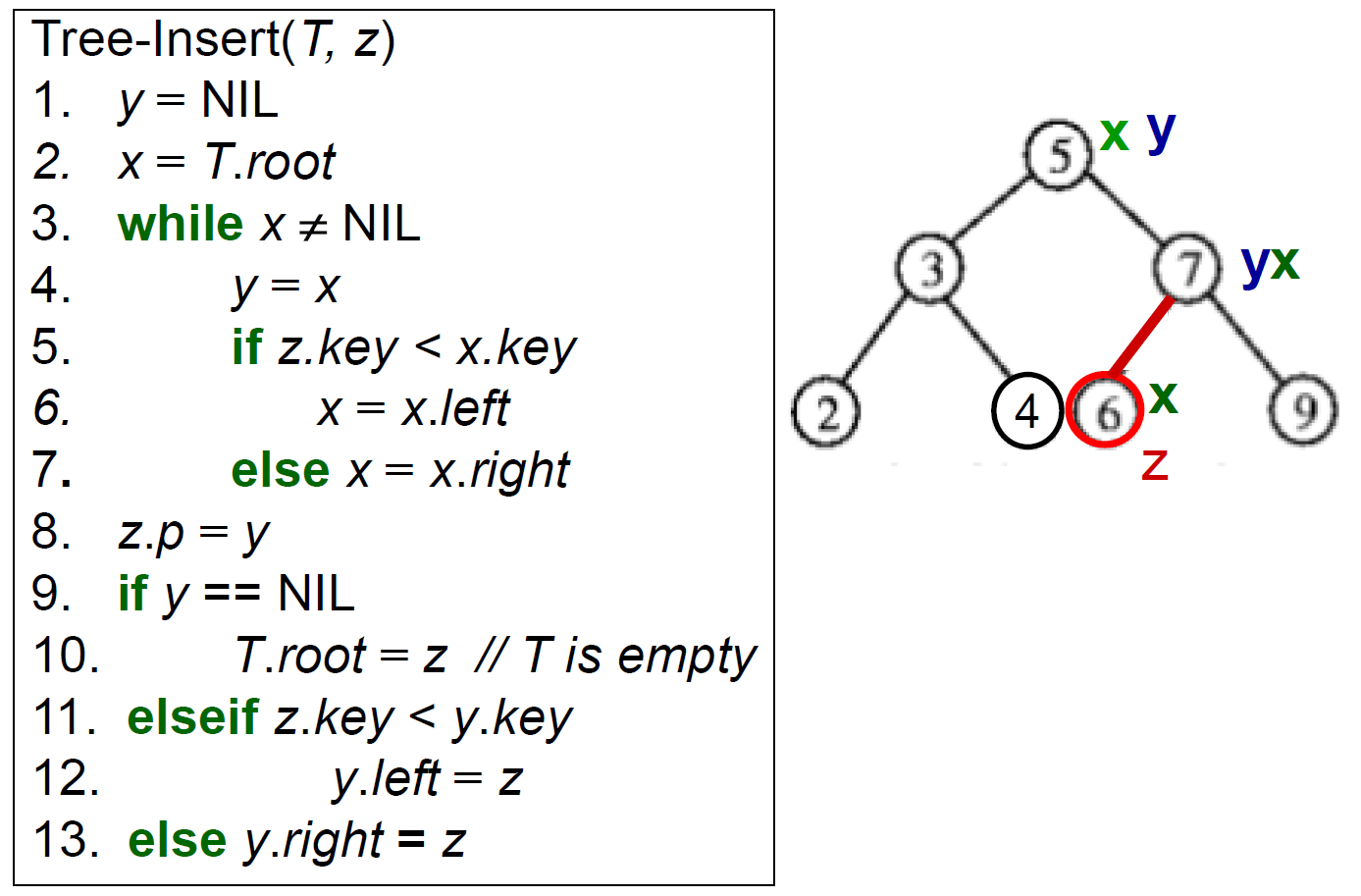
- insertion
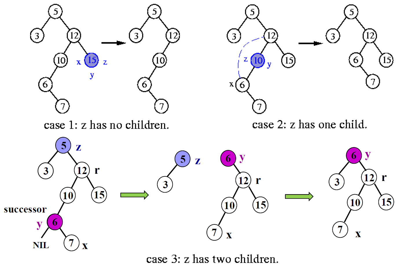
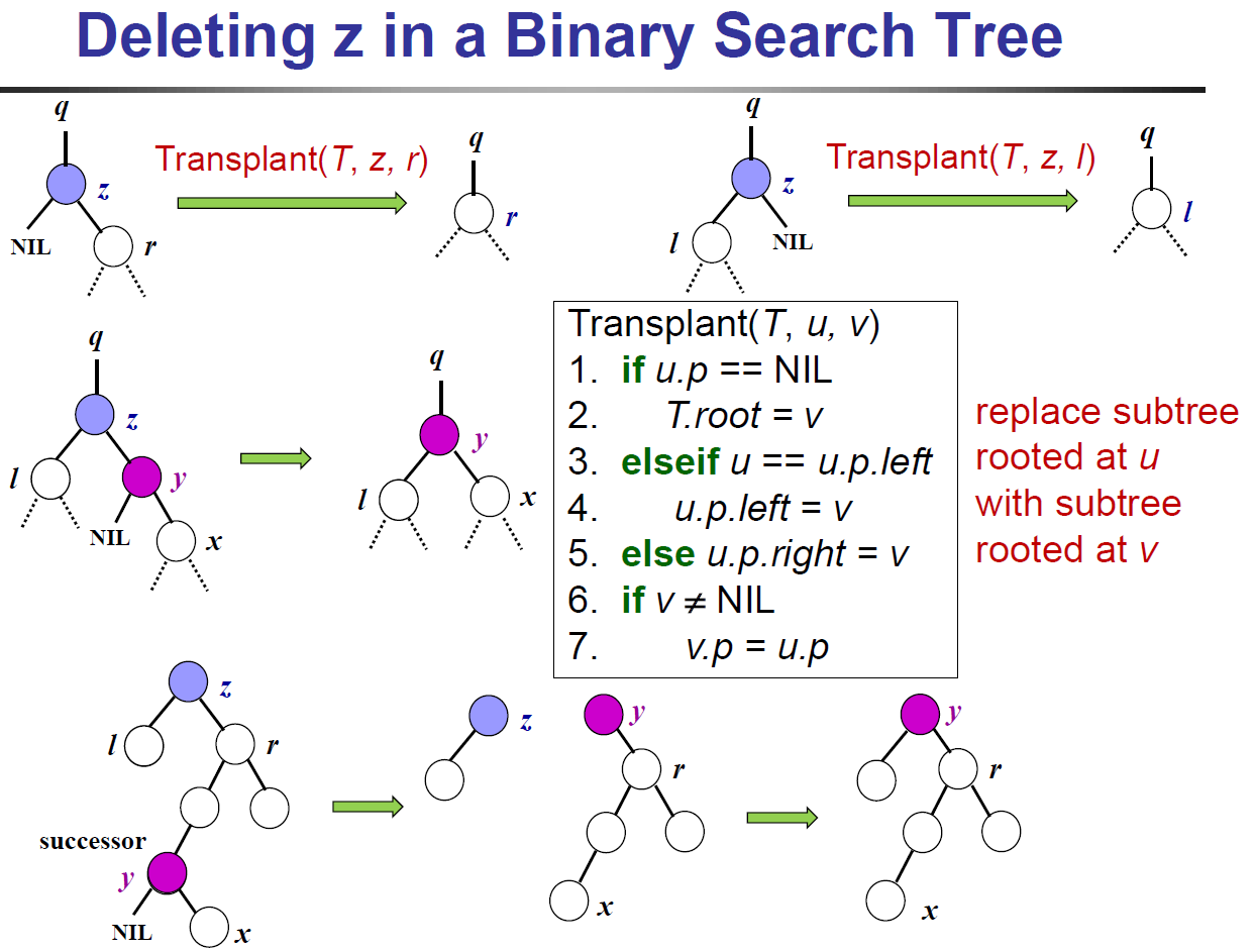
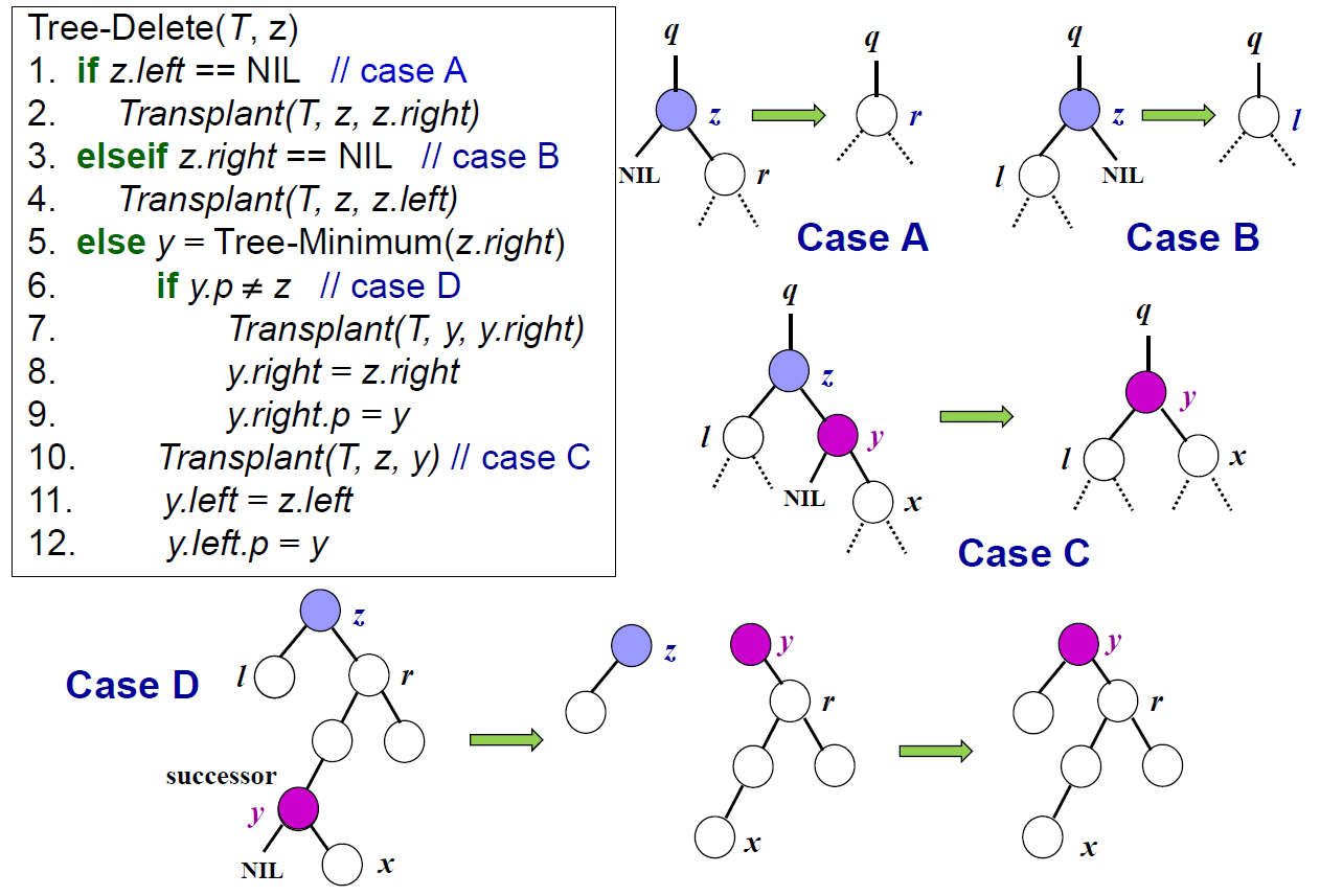
- deletion
- no children → just die
- 1 child → 小孩給媽媽養
- 2 children → 找 successor 取代
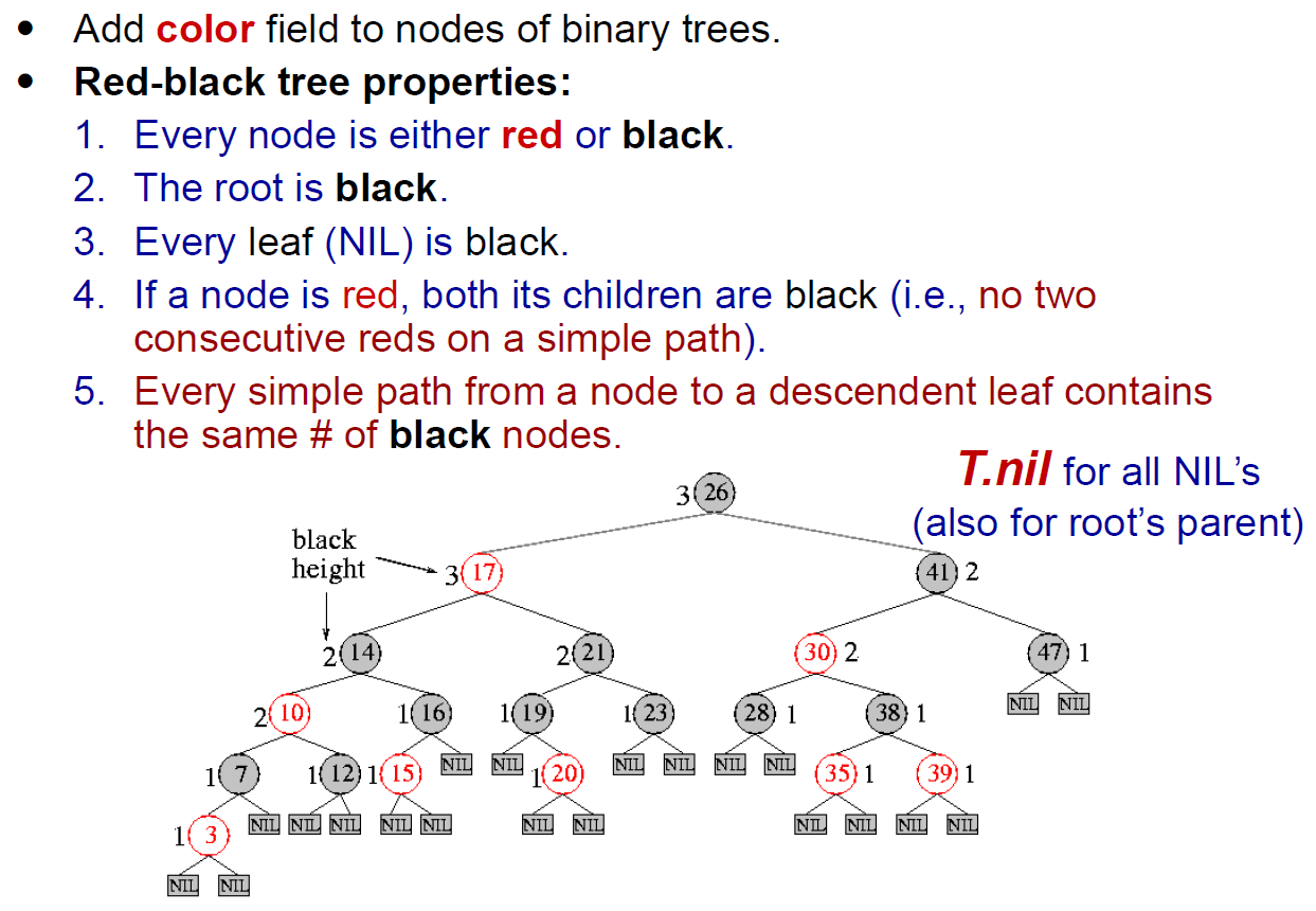
Red-Black Tree
- see Data Structure#Red-Black Tree
- black height of node x = num of blacks on path to leaf - 1 (not counting x)
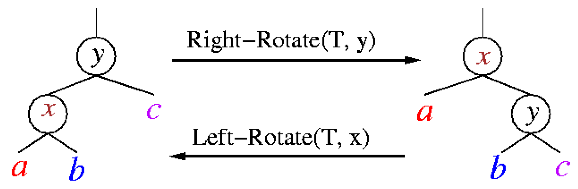
- rotation
- inorder preservation
- doubly black 指的是 deletion 後 2-3-4 一個 node 空掉的狀況
Dynamic Programming
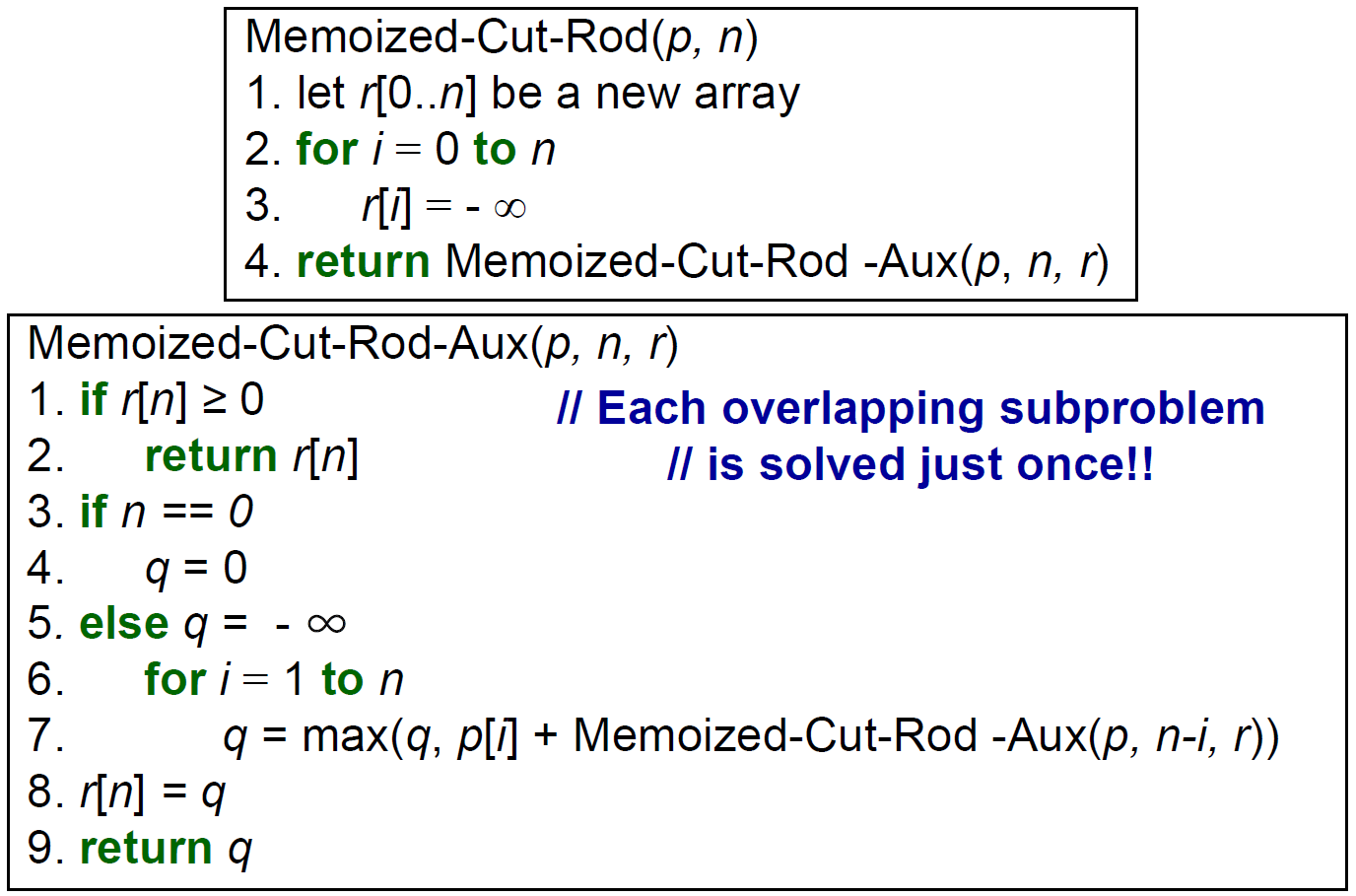
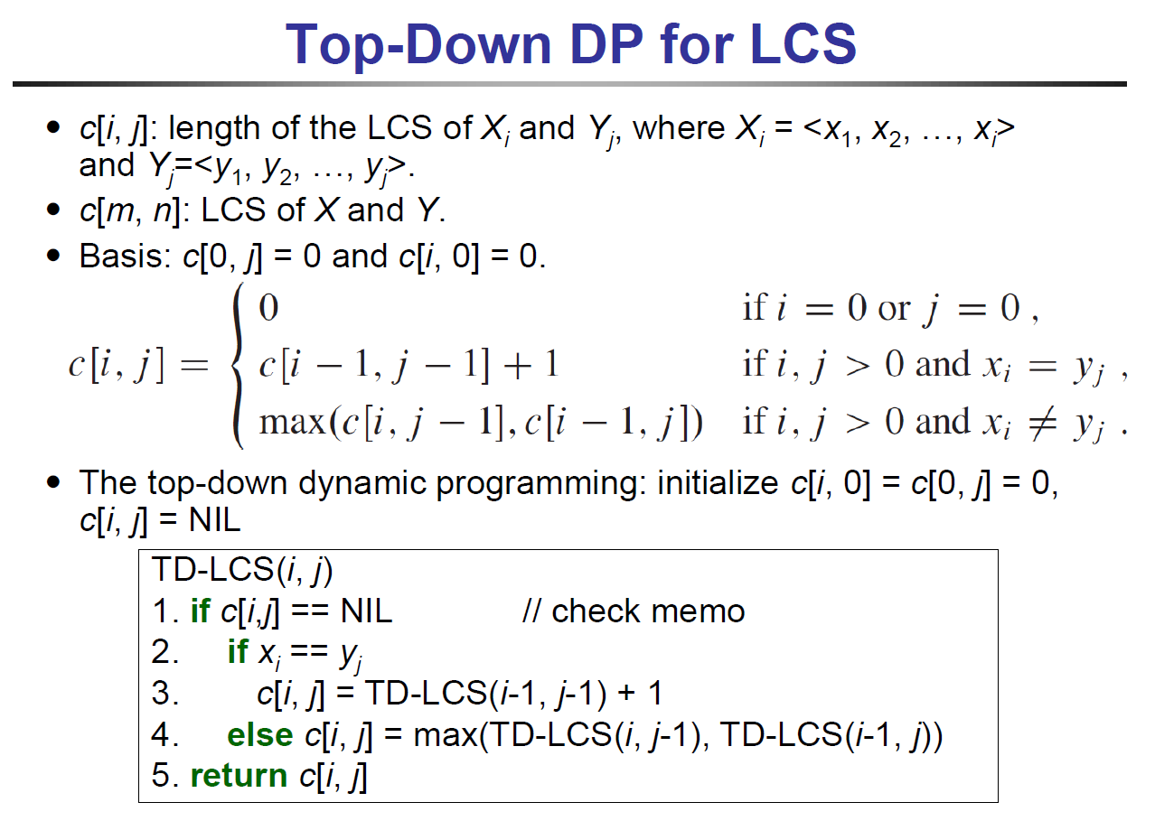
memoization
- top-down
- recursive but 記錄那些被執行過了,if 執行過則 skip
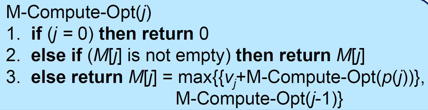
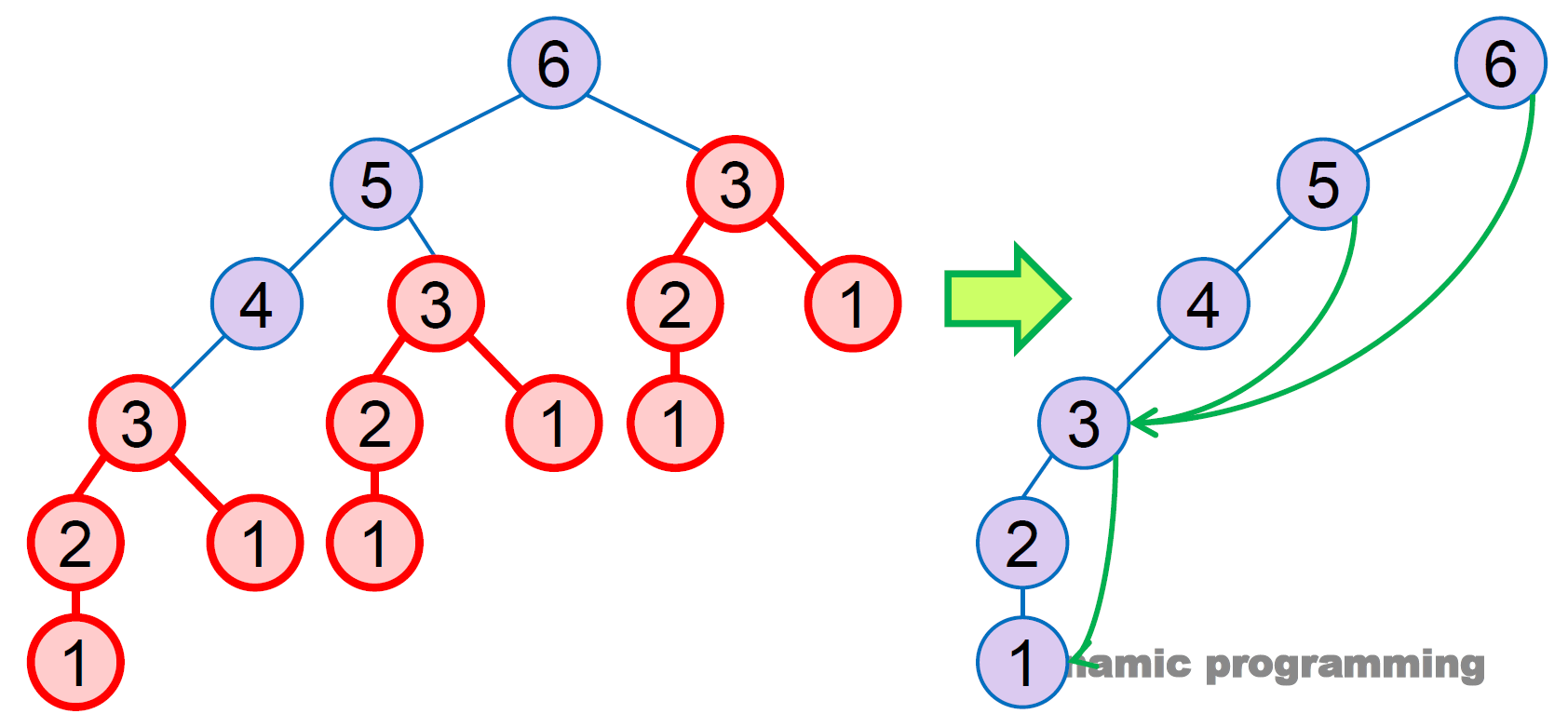
- 其實是走右邊的 3
- pros
- 不一定沒個 subproblem 都要算
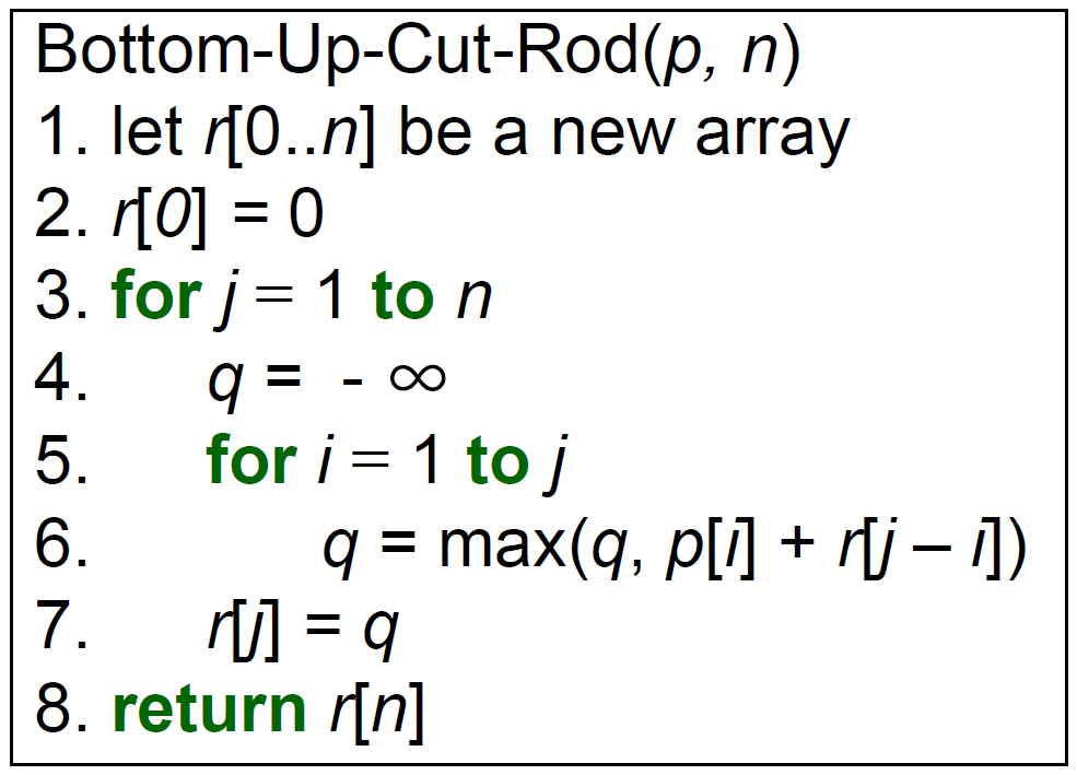
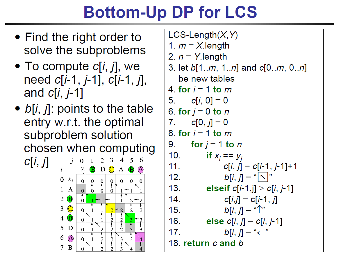
iteration
- bottom-up
- Data Structure#Dynamic Programming
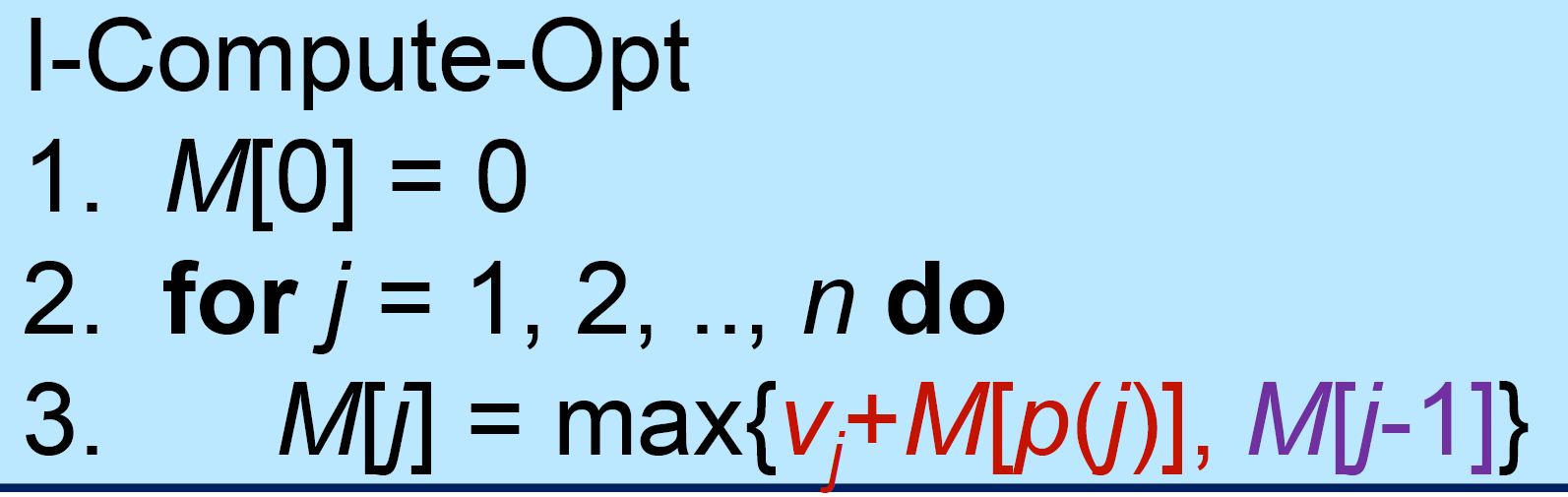
- pros
- less overhead
keys
- 適合用在 optimization problem
- 有目標的 problem
- distinct subs (table size) \(\in\) polynomial
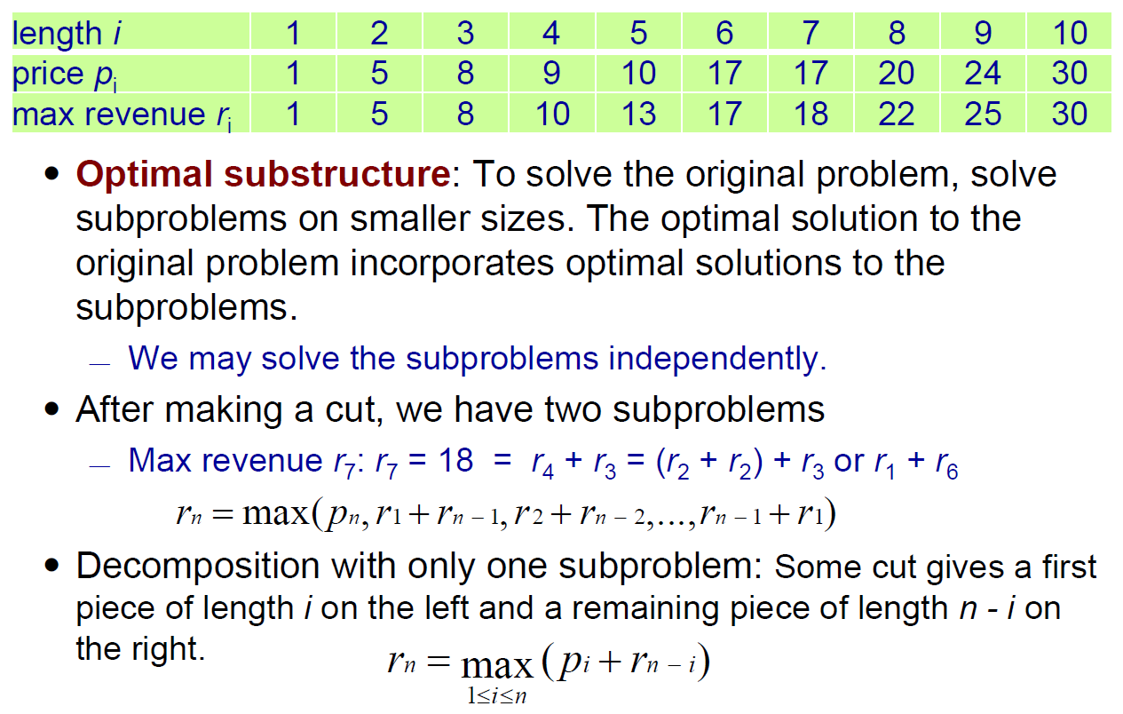
- optimal substructure
- optimal subs → optimal overall solution
- overlapping subproblem
- 很多 overlap 的 subproblems
weighted interval scheduling
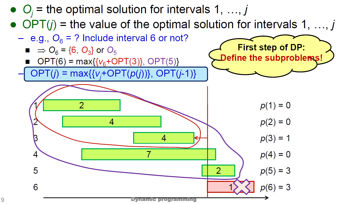
- p(j) = largest i < j s.t. i & j are disjoint
- sort by finished time
- jth 的最佳解 = max{包含 j 時的最佳解, 不包含 j 時的最佳解 i.e. j-1 的最佳解}
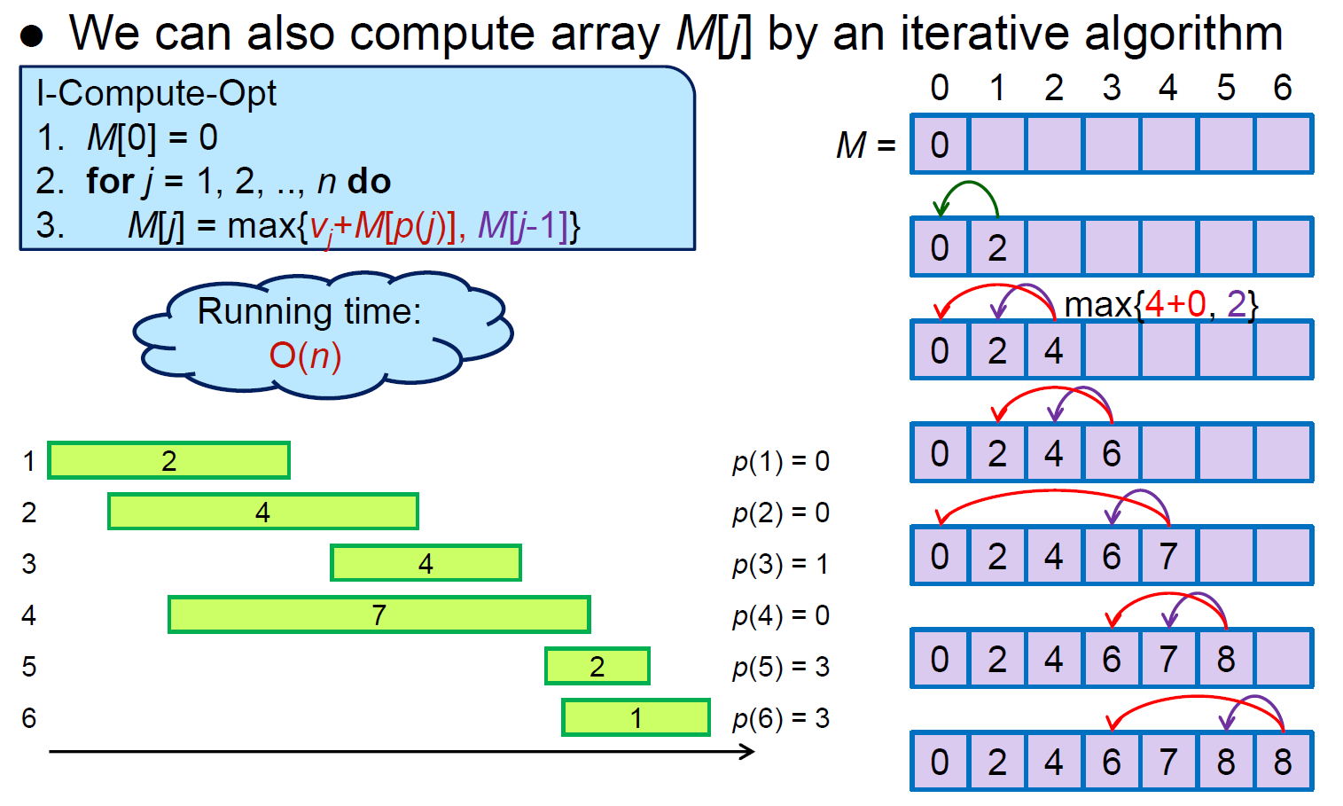
- time complexity \(\in O(n)\)
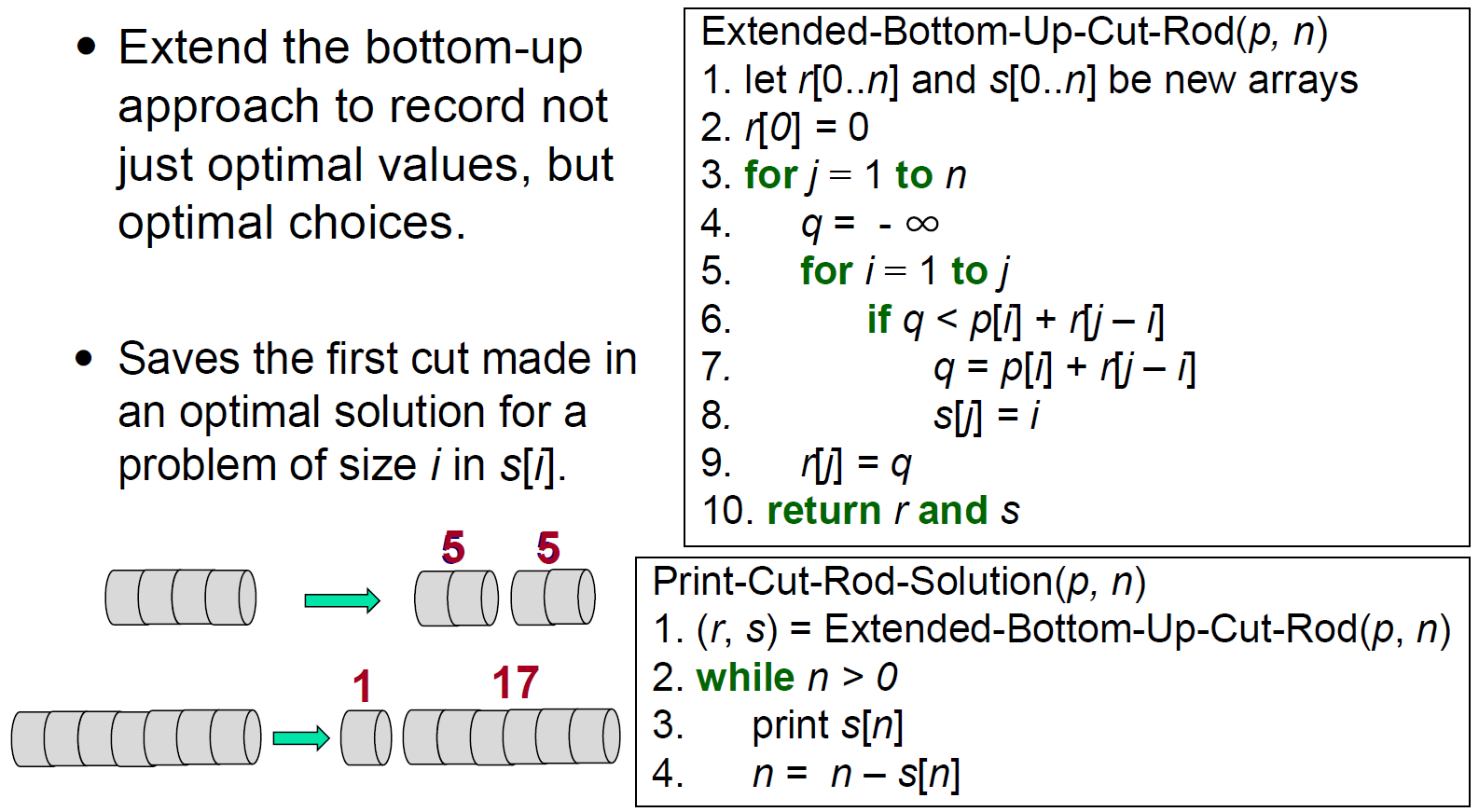
Rod Cutting
- 鋼條長度 vs. 價格非線性,求 max revenue 切法
- top-down
- \(\in O(n^2)\)
- bottom-up
- \(\in O(n^2)\)
- record choice
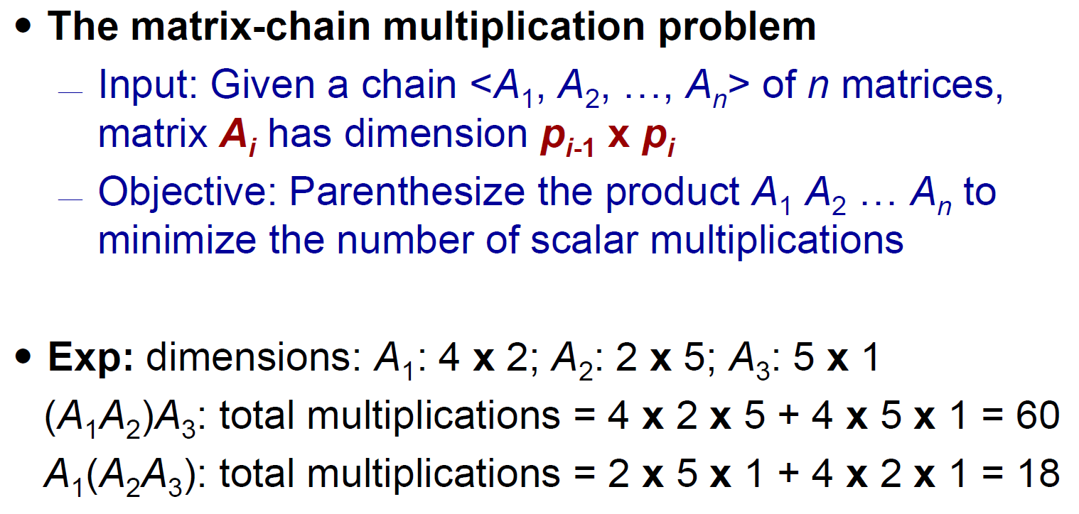
Matrix-Chain Multiplication
- minimize multiplications
- (axb) x (bxc) → ac multiplications
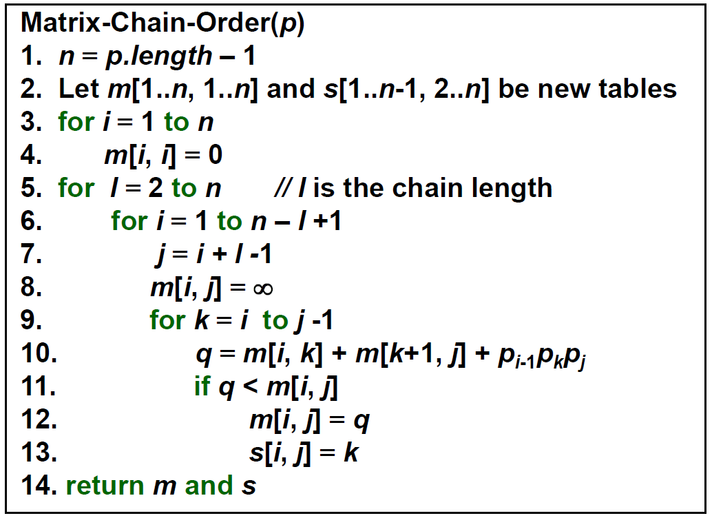
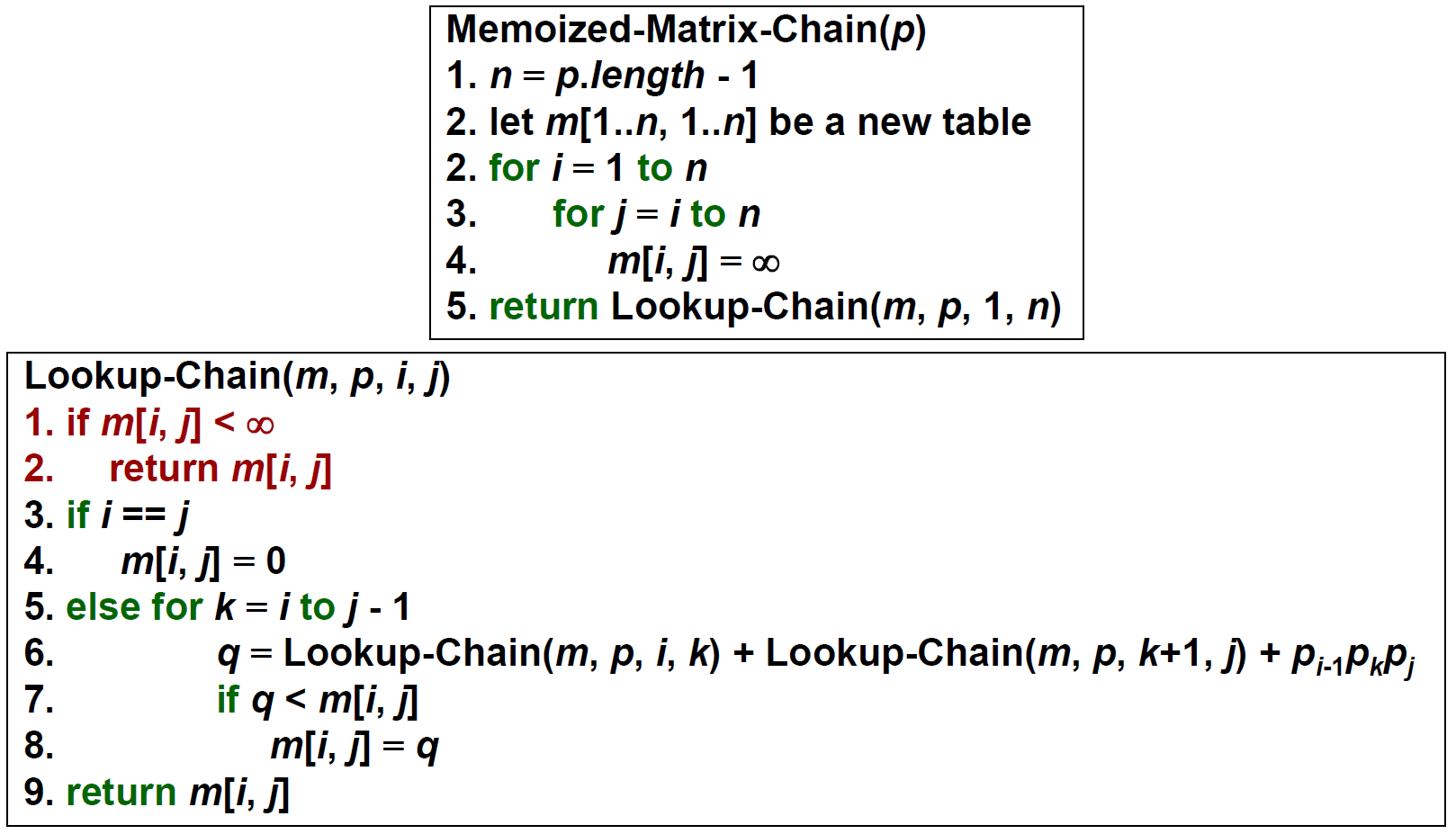
- 建立 table m,m[i, j] 記錄 \(A_i\) 乘到 \(A_j\) 的 min multiplication
- m[i, j+1] 就是 loop over 各種之間連乘對到的格子 + the rest 連乘的 cost 的 min
- time \(\in O(n^3)\)
- space \(\in O(n^2)\)
- bottom-up
- top-down
longest common subsequence
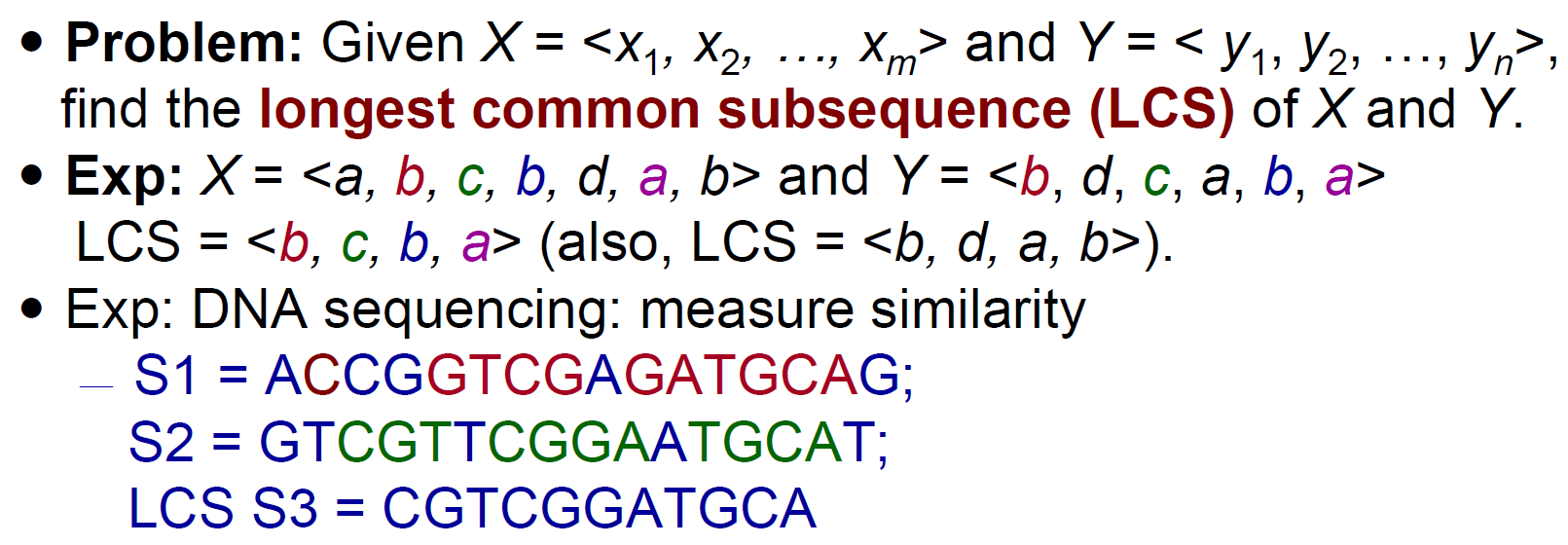
- table
- c[i,j] 表 X[1:i] & Y[1:j] 的 LCS 長度
- X.length = m, Y.length = n → c[m,n] = X Y overall LCS 長度
- top-down
- bottom-up
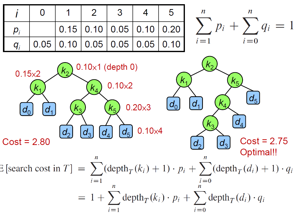
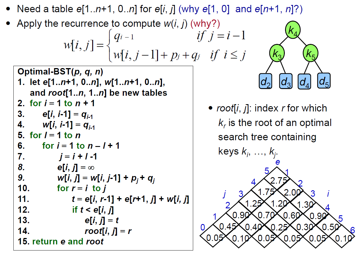
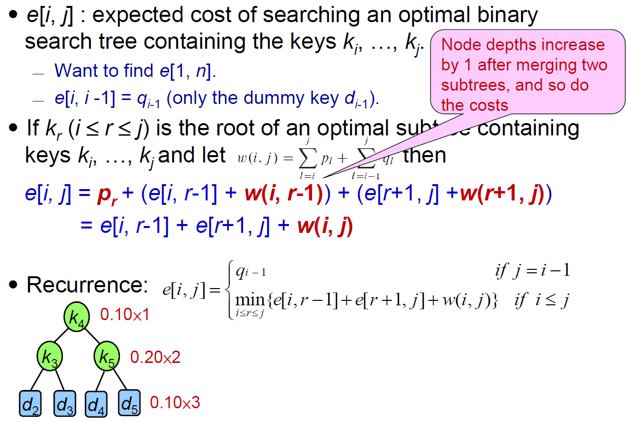
optimal Binary Tree
- binary tree with minimum expeceted search cost
- table
- p[i] probability
- probability of node i to be searched
- q[i] ==???==
- e[i,j] ==???==
- p[i] probability
Subset Sums
- NP-Complete
- 包包限重 W,給定各種不同重量的物品,怎麼塞能夠 maximize 塞的重量?
- 給定一個 set & 一個 constraint W,求 max subset 的 sum <= W
- table m = n x W
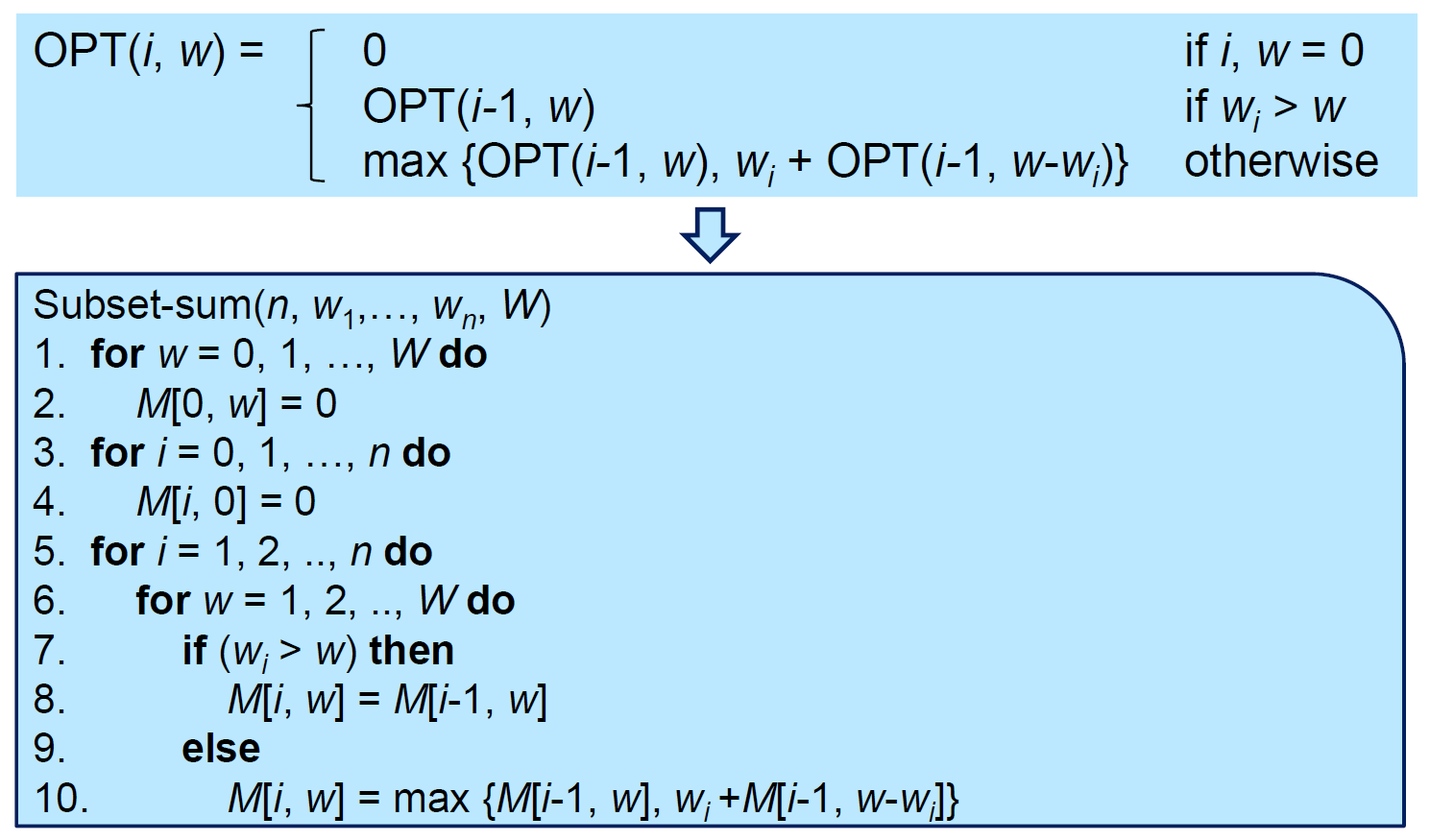
- max(沒自己, 有自己)
- w 剩餘可用的 weight
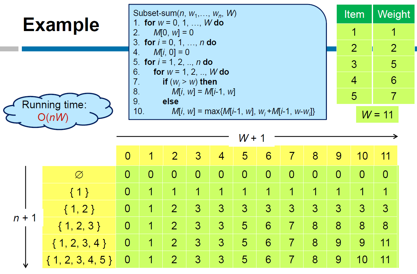
- e.g.
- time complexity \(\in O(nW)\)
- pseudo-polynomial
- W may not be polynomial to n
- pseudo-polynomial
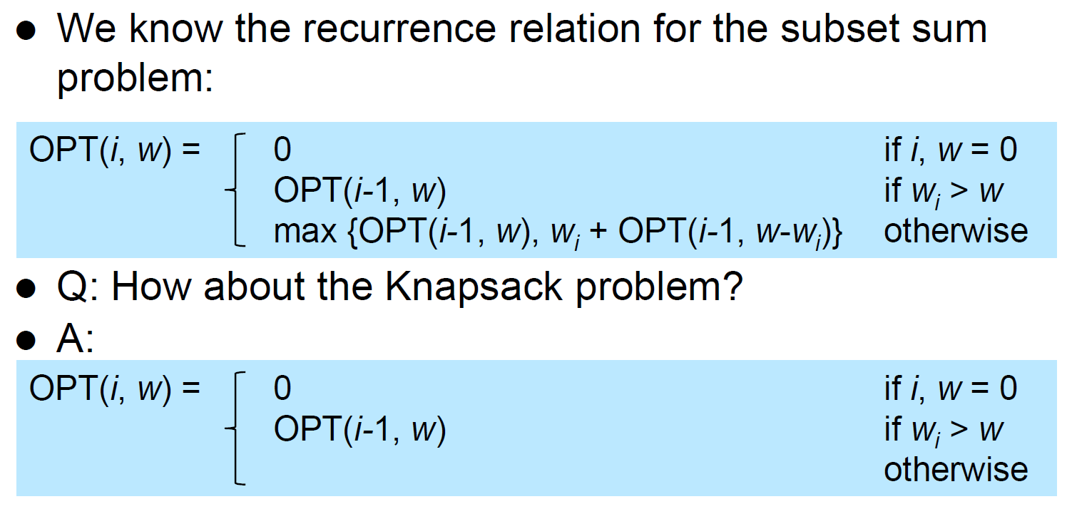
Knapsacks
There are \(n\) items with values \(v_1\) to \(v_n\) and weight \(w_1\) to \(w_n\).
The max total value attainable from the first \(i\) items for a bag with weight limit \(w\) = \(dp(i, w)\) =
- \(\max(dp(i-1, w), v_i+dp(i-1, w-w_i))\) if \(w>=w_i\)
- \(dp(i-1, w)\) else
time & space complexity = \(O(nW)\) where \(W\) is the weightcapacity
- #Subset Sums problem but each item has a value and the goal is to maximize the total value
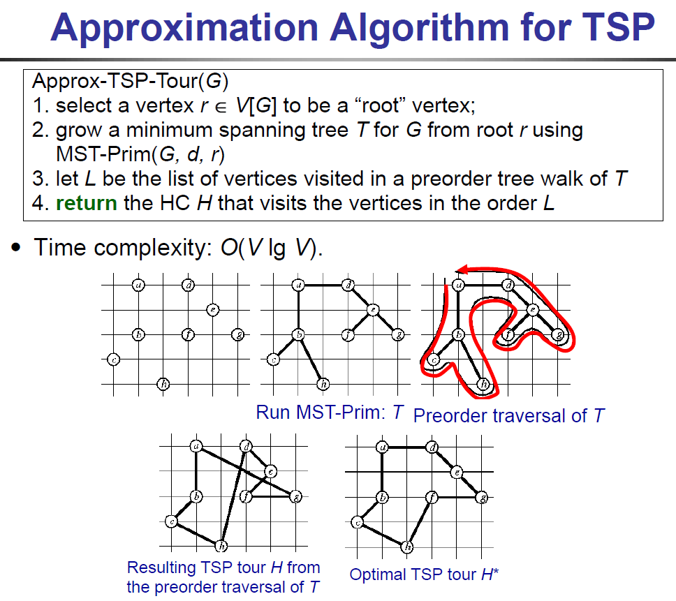
Traveling Salesman Problem
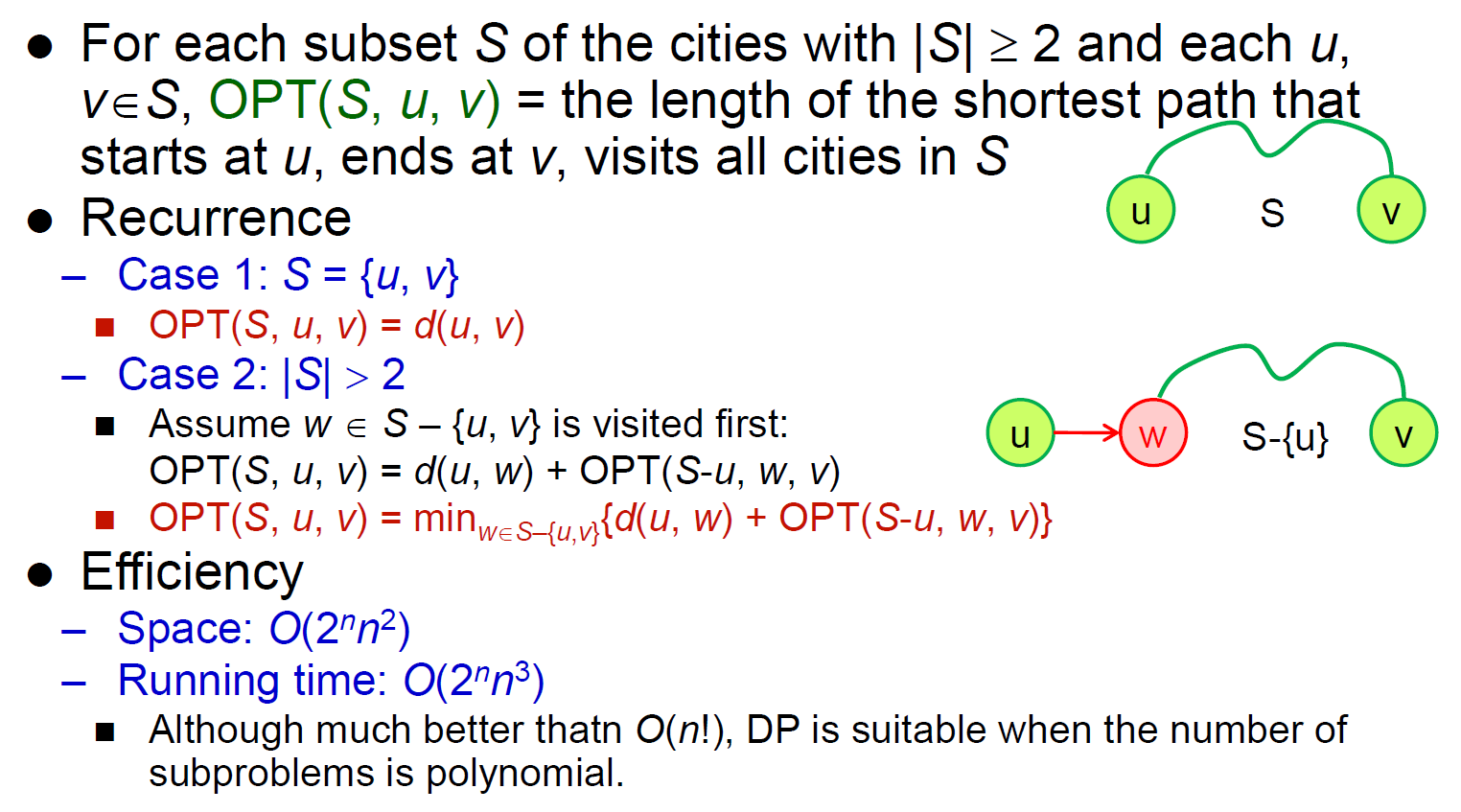
- space \(\in O(2^nn^2)\)
- runtime \(\in O(2^nn^3)\)
Greedy
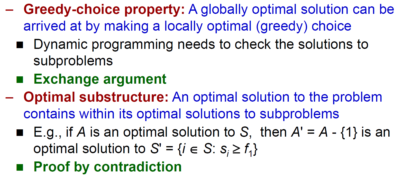
properties
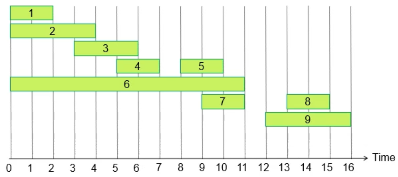
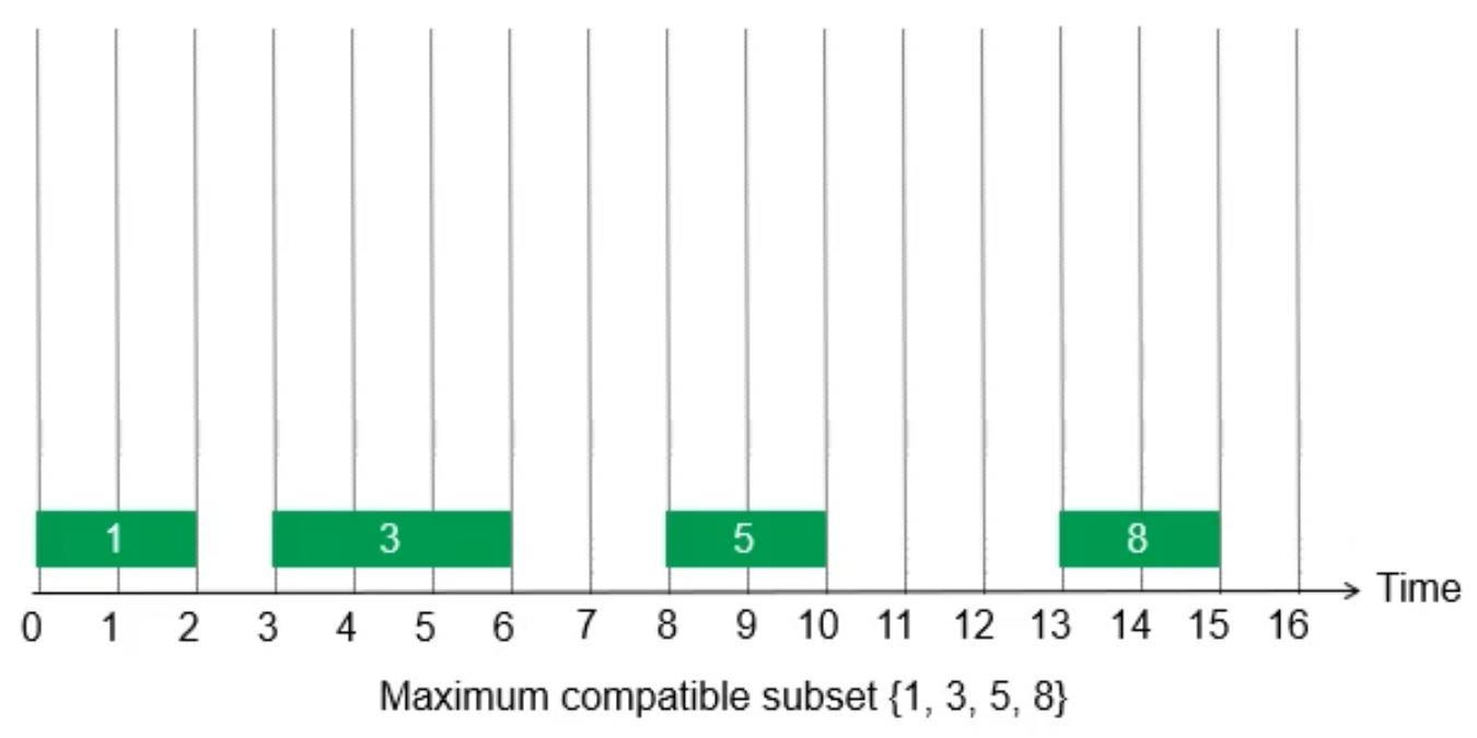
interval scheduling
- solution
- sort by finished time
- select the 1st one
- if the current one overlaps the last selected one, then omit it
- e.g.
pf
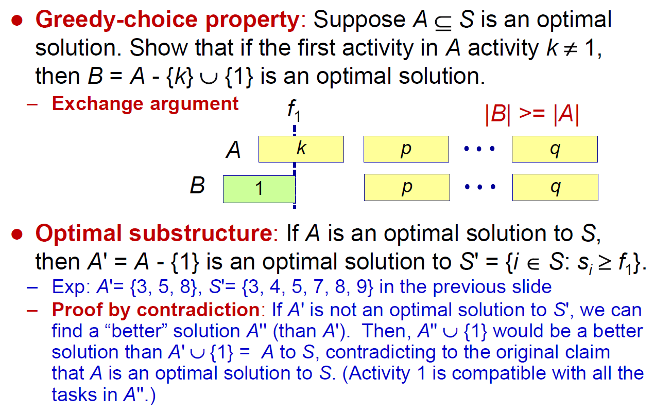 exchange → 數量一樣
comparison to #Dynamic Programming
- greedy
- top-down
- 1 subproblem
- 一定也能用 dynamic programming 解
- dynamic programming
- bottom-up
- several subproblems
Huffman codes
- https://iq.opengenus.org/huffman-coding-vs-fano-shannon-algorithm/
- characters represented by binary string
- fixed-length code (block code)
- 3 bits a character
- a-f
- variable-length code
- less bits for more frequent ones
- prefix code
- no code is a prefix of some other codes
- binary search tree
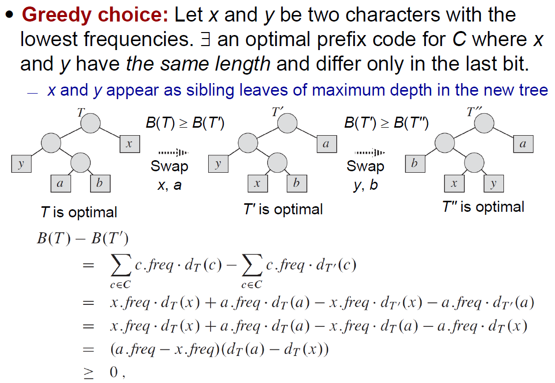
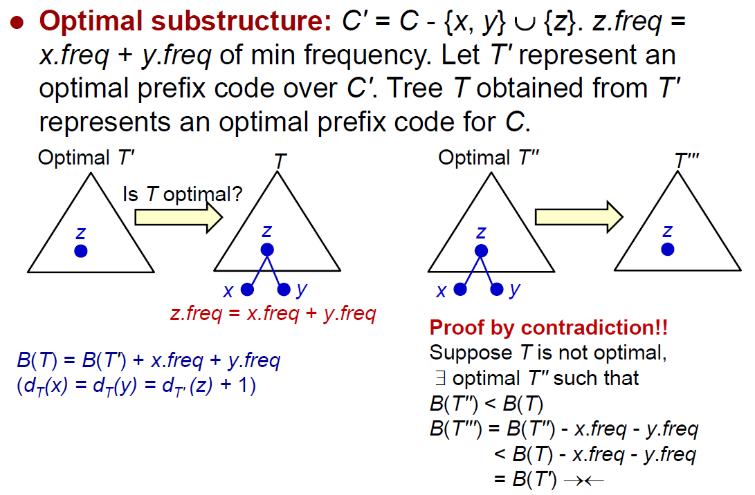
- 每輪把 frequency 最低者 pair 在一起 → 最後 frequency 最低者會沉在最下面
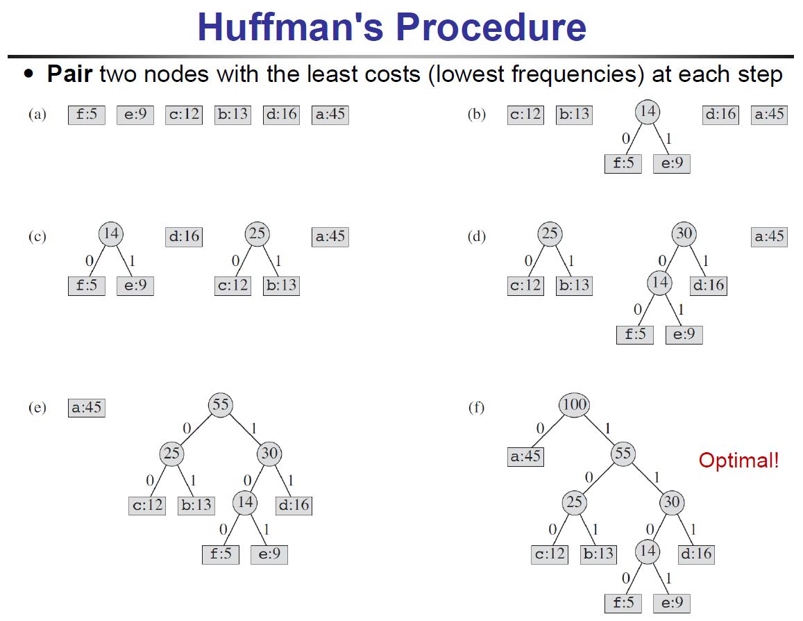
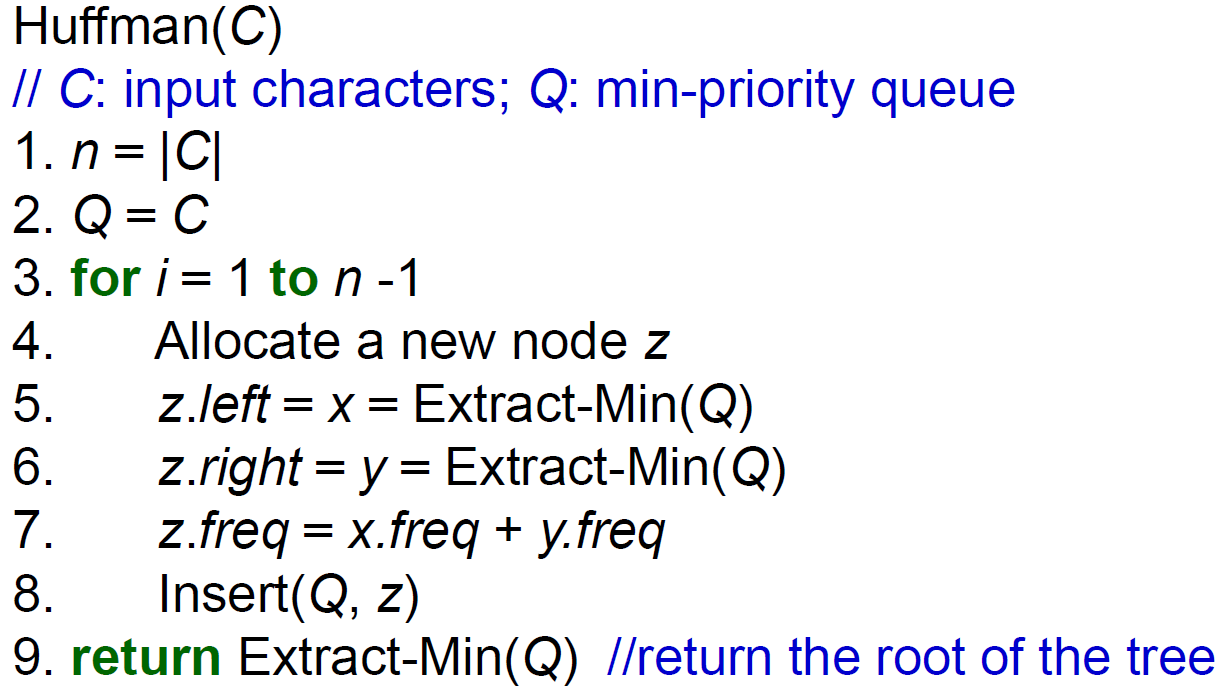
- time complexity \(\in O(nlgn)\)
- greedy properties
task scheduling
- n 個需要花時間 1 單位時間完成的 tasks
- \(N_t(A)<=t\)
- 在 t 時間內能夠完成的 tasks 數不超過 t
Graph
- \(V\) nodes (vertexes)
- n nodes
- node.d = discovery time of node
- node.f = finishing time of node
- node.\(\pi\) = parent of node
- \(E\) edges
- m edges
- undirected
{u,v}
- directed
(u,v)
- path
- simple path
- all nodes are distinct
- cycle
- simple path
- connectivity
- there is a path for every pair of nodes in this graph → connected
notations
- node.d = distance from source node
- node.\(\pi\) = parent of node
graph representation
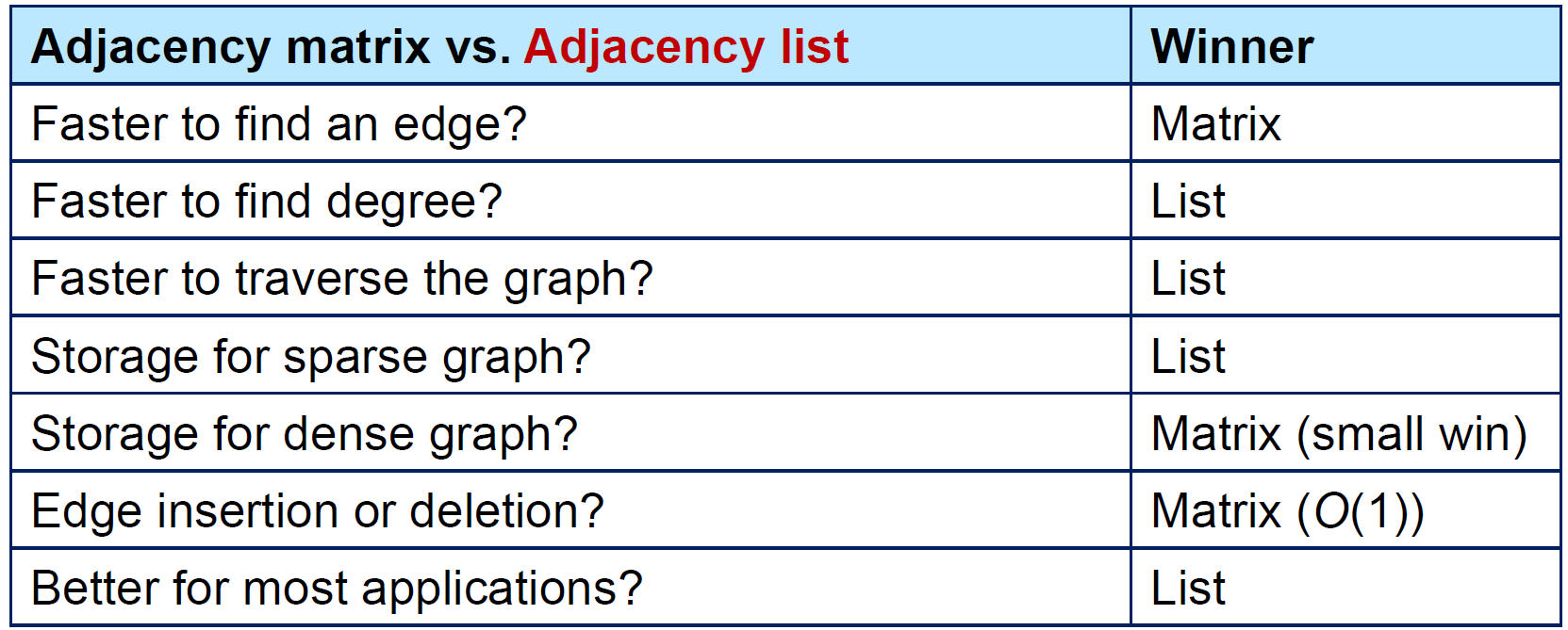
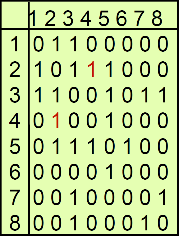
adjacency matrix
- 存 edge
- 查看任兩點有沒有相連 → 一格 → constant time
- 找一點有幾個 neighbor → 1 row → O(n)
- space \(\in O(n^2)\)
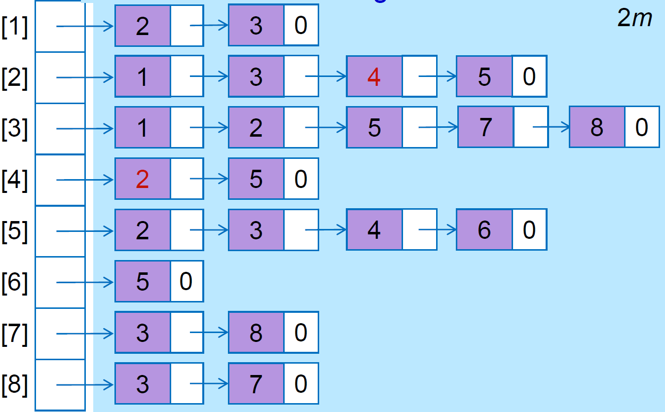
adjacency list
- 存 node
- 放該 node 的 neighbors
- \(O(deg(u))\) for 檢查是否為 neighbor
- deg(u) = amount of u's neighbors
- space \(\in O(n+m)\)
graph traversal
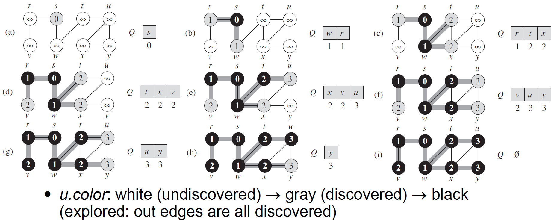
BFS
- breadth-first-search
- 先走完所有 neighbor 再往下走
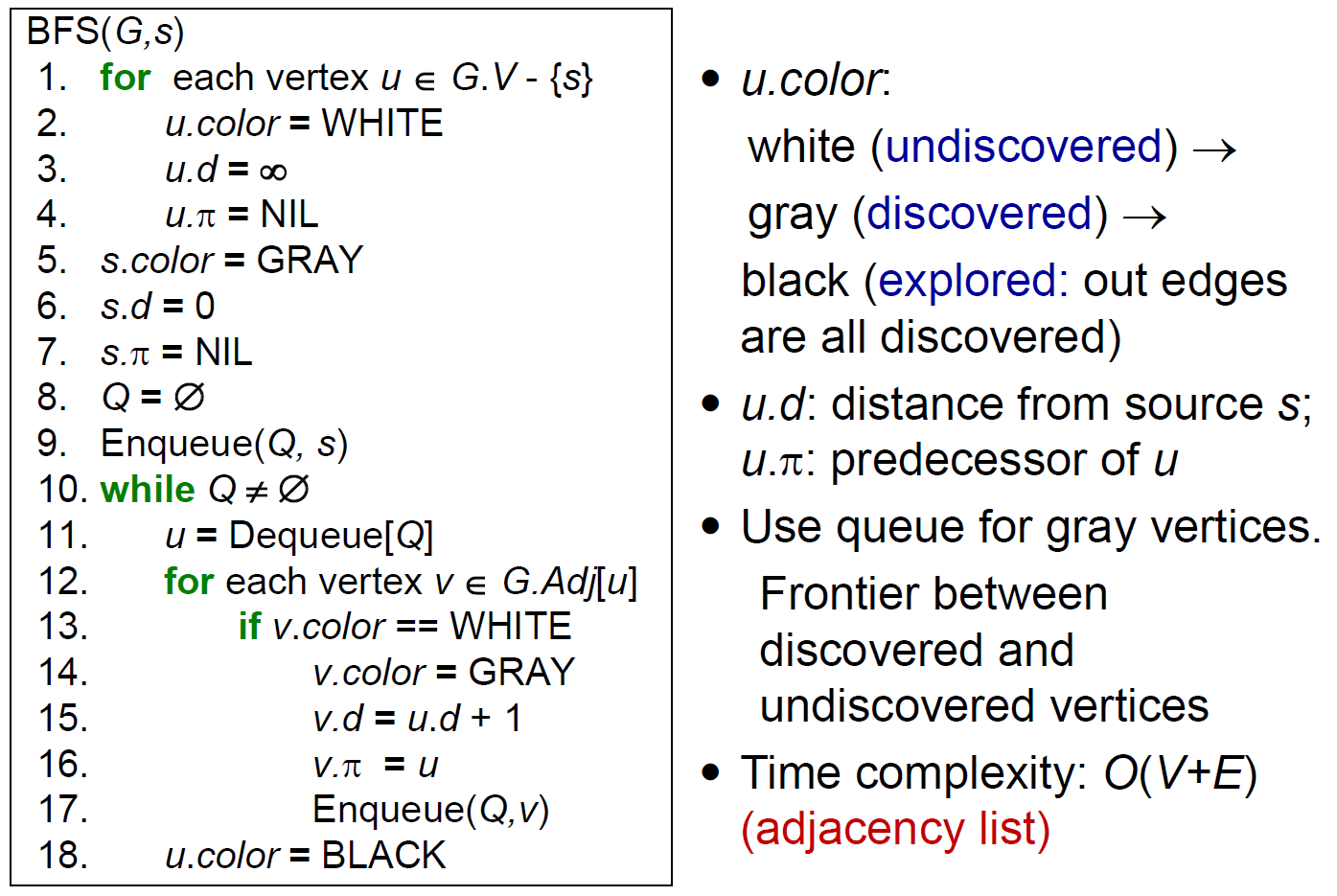
- e.g.
- time complexity \(\in O(V+E)\)
- each vertex enqueued & dequeued once
- each edge considered once
DFS
- depth-first search
- 先走到底再走鄰居
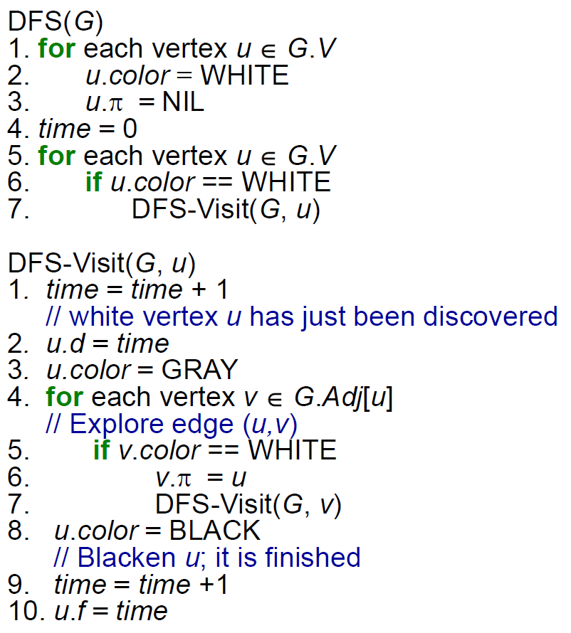
- 經過 → grey
- retreat → black
- e.g.
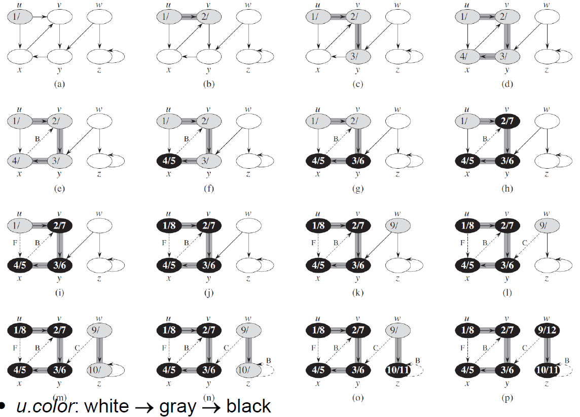
- 圖中有標示 edge type
- parenthesis property
- if u is v's descendant,經過順序會是 v → u → u → v
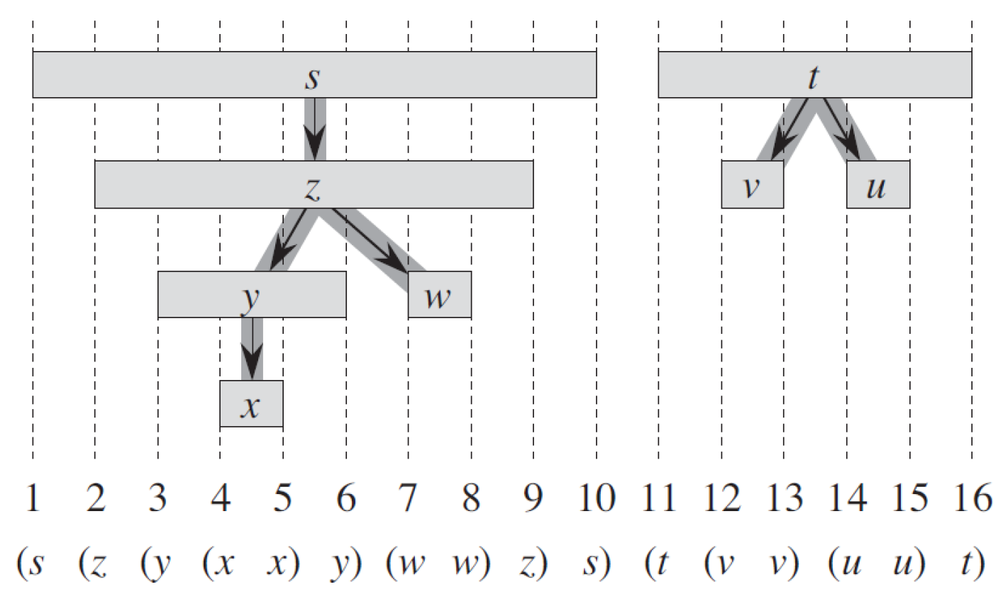
- 因為會 retreat
- edge type
- directed graph
- tree edge
- DFS 後的一般 edge
- if 指到 white (not discovered)
- back edge
- descendant 指到 ancestor
- 出現 cycle
- if 指到 grey (already discovered)
- forward edge
- ancestor 指到 indirect descendant (為 nontree edge)
- if 指到晚輩 black (already completed)
- cross edge
- 非直系血親 (為 nontree edge)
- if 指到非晚輩 black (already completed)
- tree edge
- undirected graph
- tree edge
- back edge
- no forward edge
- forward edge = back edge in undirected graph
- no cross edge
- 沒有 ancestor or descendant 關係 → 無法判斷是否為旁系
- directed graph
DAG
- directed acyclic graphs, directed graphs without cycles
- undirected graph without cycle → tree / forest
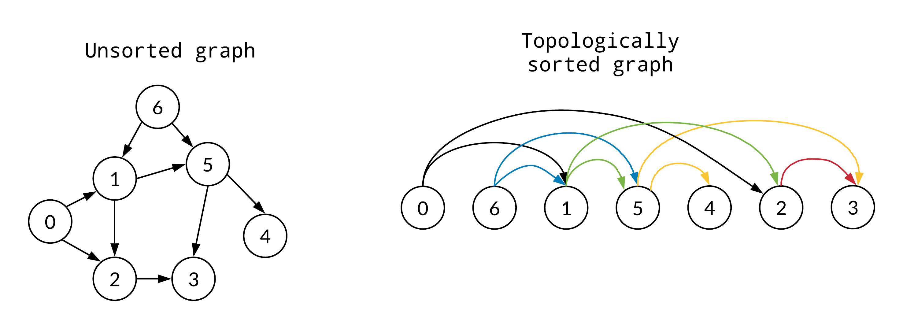
- topological ordering
- nodes 排成一條線,edge 的方向一致
- 找法:從沒有 incoming edge 者開始
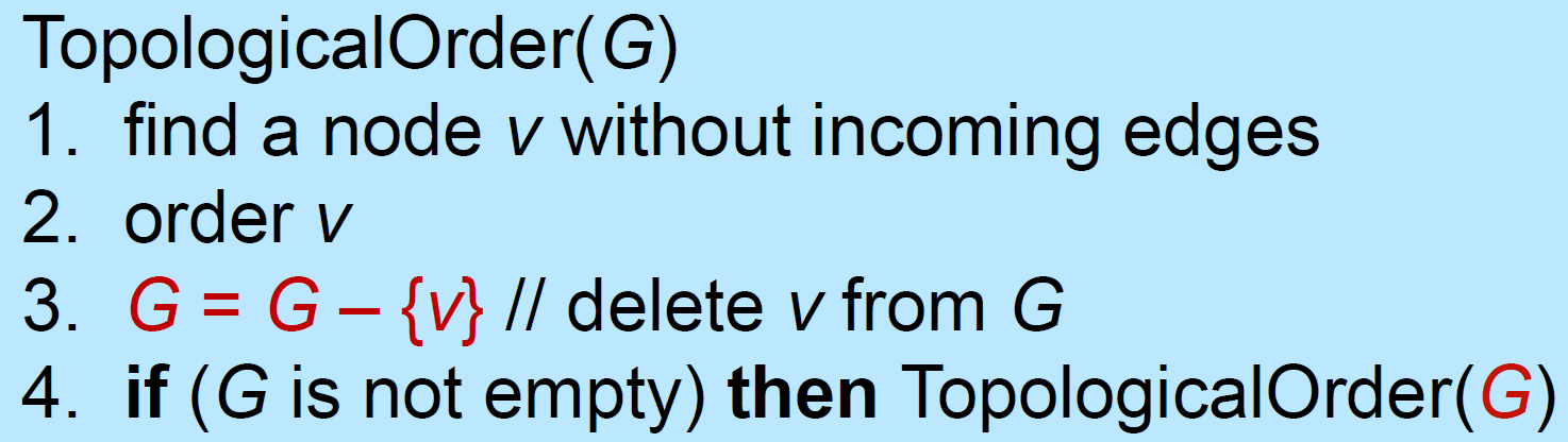
- time complexity \(\in O(n^2)\) to \(O(m+n)\)
- e.g.
- has topological ordering iff is DAG
- topological sort
- sort nodes in decreasing finishing time
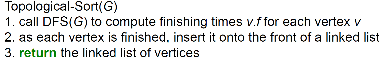
- time complexity \(\in O(V+E)\)
connectivity in directed graph
- every node is mutually reachable → the graph is strongly connected
- every node is mutually reachable ignoring the direction of edge → the graph is weakly connected
SCC strongly connected component
- SCC of s = maximal set of v s.t. s & v are mutually reachable
- for any 2 nodes s & v in a directed graph, their strongly connected components are
- identical if s & v are mutually reachable
- disjoint if s & v aren't mutually reachable
- SCC of a directed graph G=(V, E) = maximal set of node \(U\in V\) s.t. u→v & v→u
- https://www.geeksforgeeks.org/strongly-connected-components/
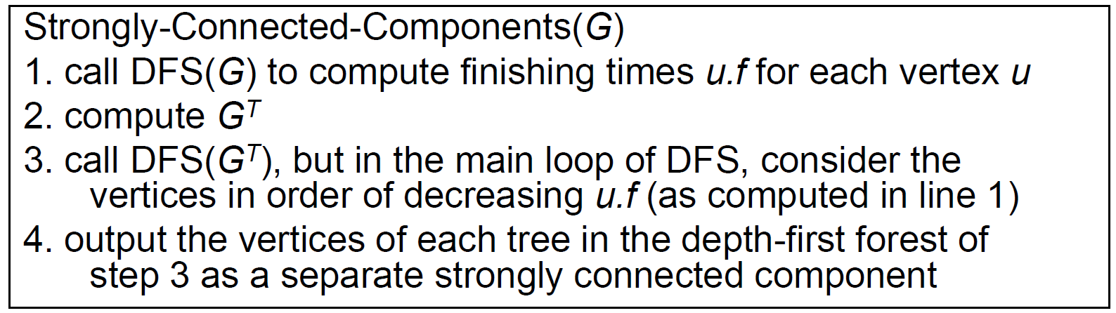
- time complexity \(\in O(V+E)\)
- SCC graph is a #DAG
minimum spanning tree, MST
- find edges that connect all nodes with min cost
- 不會有 cycle
- 有 cycle → 去掉連回去的那個 edge 還是會是 connected graph
- use greedy to solve
solutions
- generic
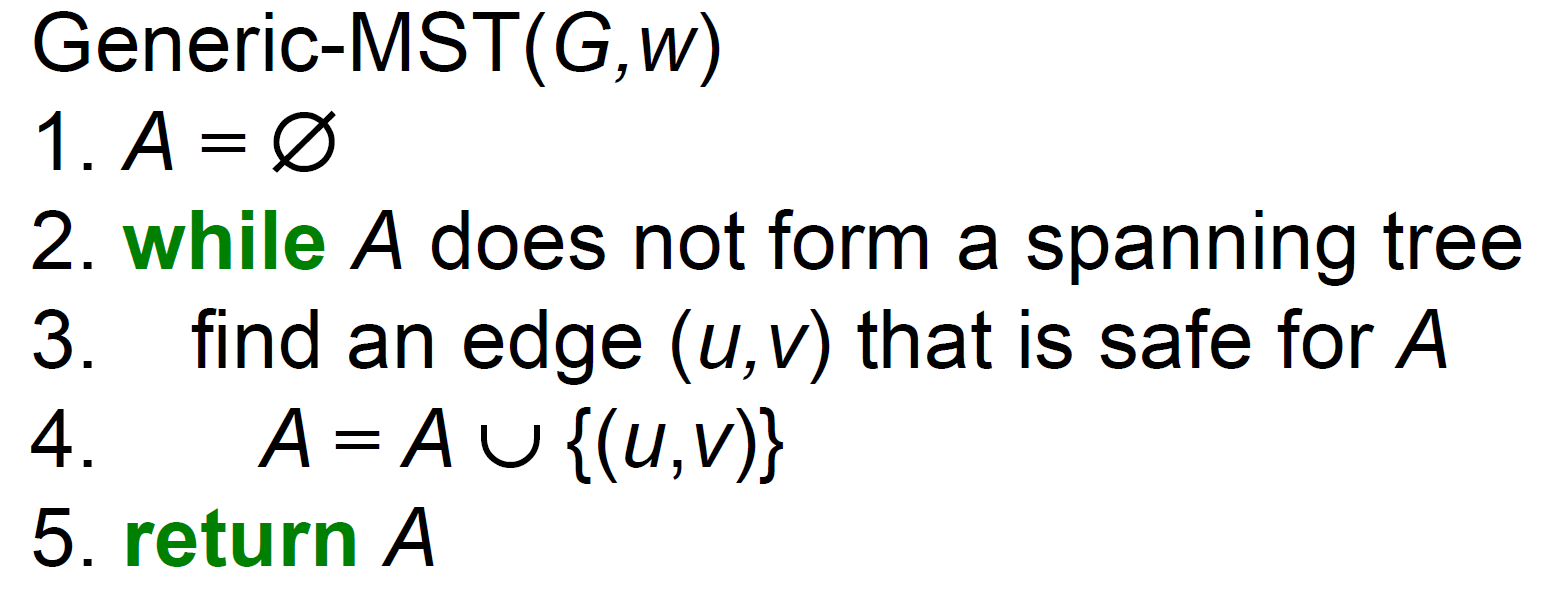
- add a safe edge every time
- 找 cut 裡最便宜的 edge
- Kruskal's algorithm
- start with no selected edge, sort edge by cost,每次都選剩下的最便宜的 edge,會 cycle 則 discard
- 每多一個 edge 就會 merge 兩個 tree
- implementation
- 每個小 tree 都是一個 disjoint set
- 新的 edge 屬於同 disjoint set → cycle
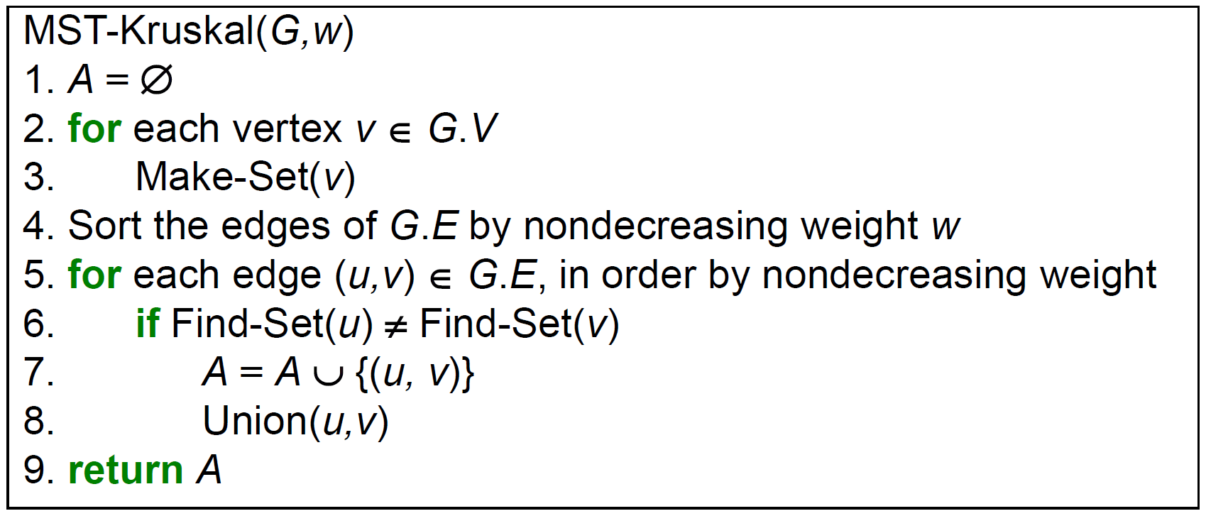
- time complexity \(\in O(ElgE+V)=O(ElgV+V)\)
- find-set for a set of V nodes = \(\alpha(V)\)
- for each edge → \(O(E\alpha(V))\)
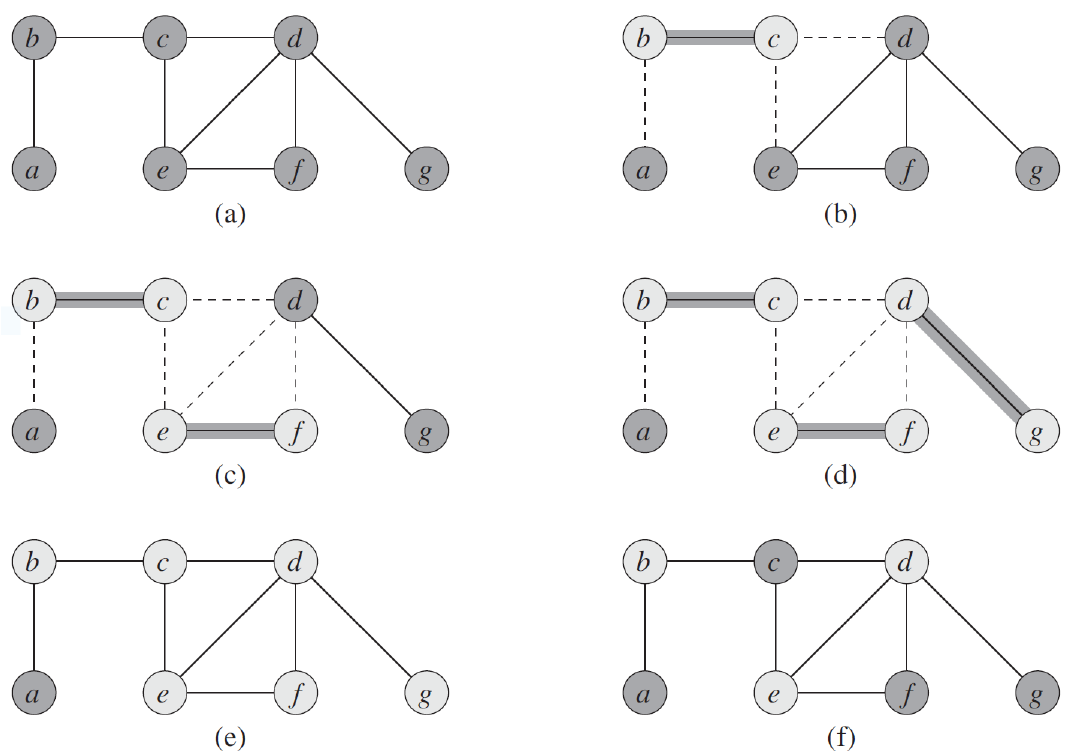
- Prim's algorithm
- start with root node, greedily expands outward from the current tree
- implementation
- 用 heap 找最便宜的 cut
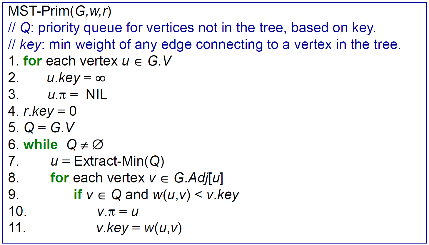
- 先把所有 key 設 infty
- root 的 key 為 0
- heap 存所有 nodes
- 更新 min node 連到的所有 node 的 key
- \(\pi\) for 路徑
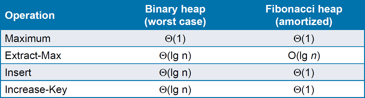
- time complexity
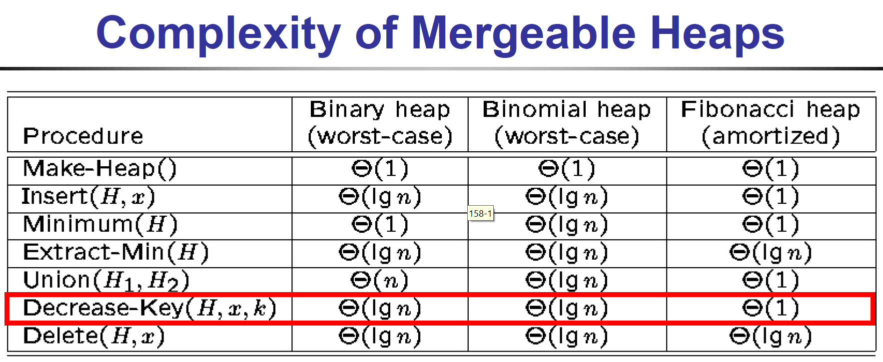
- \(O(ElgV)\) with binary heap
- \(O(E+VlgV)\) with Fibonacci heap
- reverse-delete algorithm
- reverse of Kruskal's algorithm
- start with all edges selected, sort edge by cost, delete the max cost edge, skip if it would disconnect the graph
properties
- cut property
- a MST must contain the min cost edge than connects S & V-S for all subset S
- pf
- assume spanning tree T doesn't have the min cost edge (u,v) that connect S & V-S, if we replace the edge connecting S & V-S with (u,v), we'll have a smaller cost
- cycle property
- for any cycle,cycle 裡最貴的 edge 不屬於任何 MST
optimal substructure
- unweighted shortest path
- have optimal substructure
- unweighted longest path
- don't have optimal substructure
- e.g.
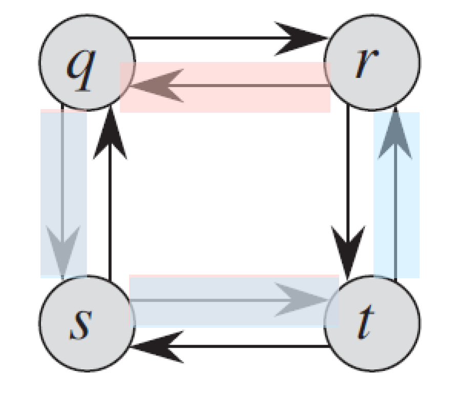
- longest path simple path of q → t is q → r → t
- longest path simple path of q → r is q → s → t → r
- longest path simple path of r → t is r → q → s → t
- shortest path
- subpaths of shortest paths are shortest paths
SSSP
- single-source shortest path
- shortest path from source node s to every other nodes
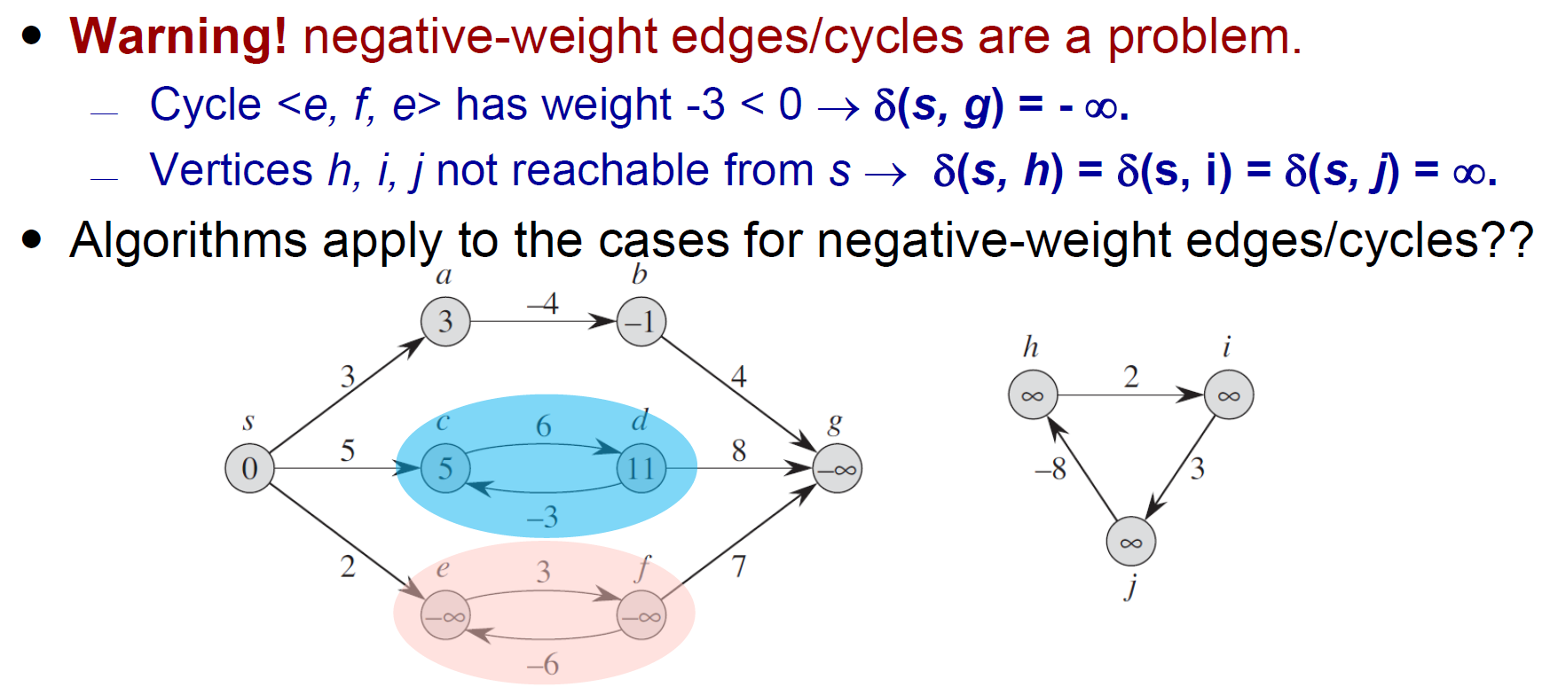
- if have negative edges
- negative cycle → 使 node cost 變成 -infty
- negative cycle → 使 node cost 變成 -infty
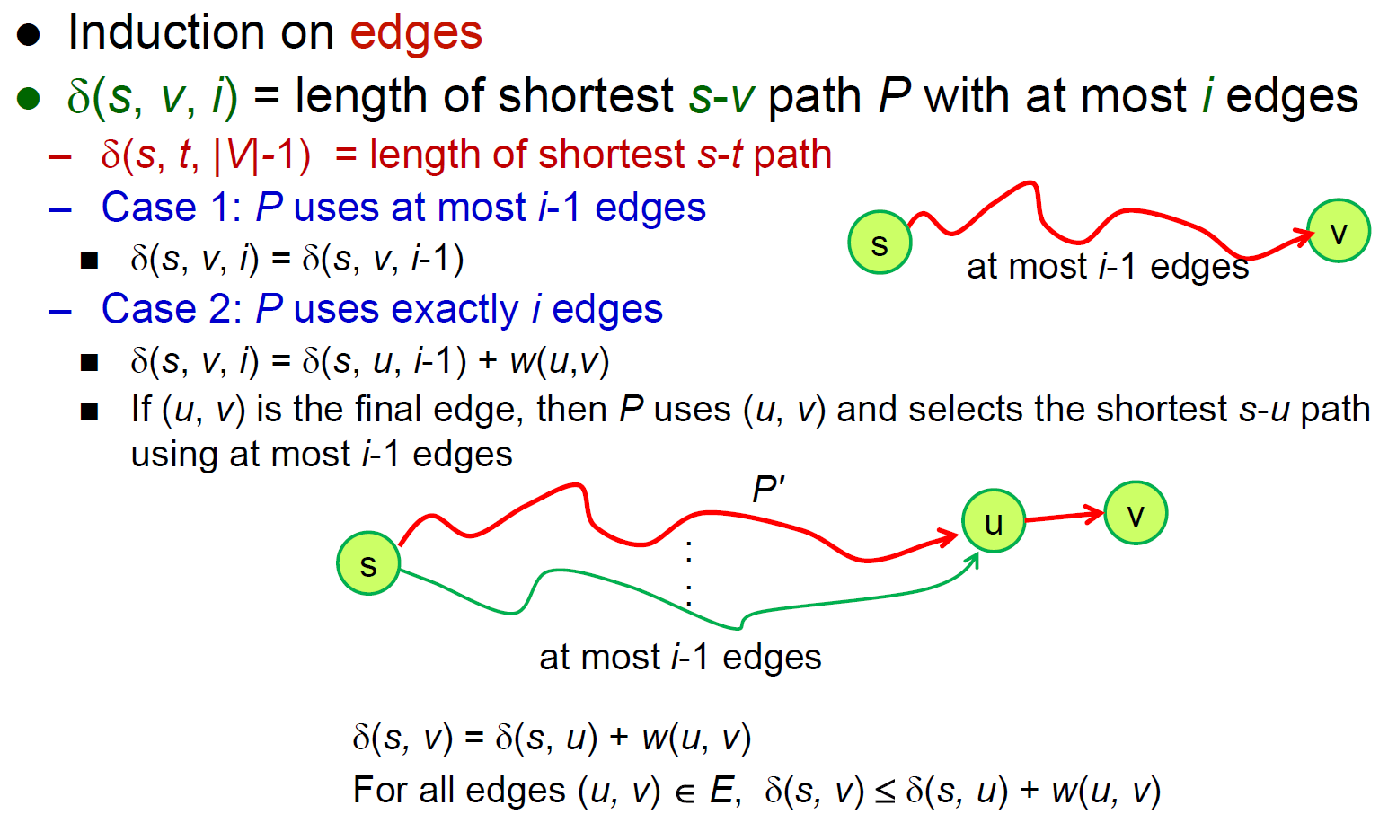
- triangular inequality
- s to u \(\leq\) s to v to u
- relaxation
- 更新 node cost
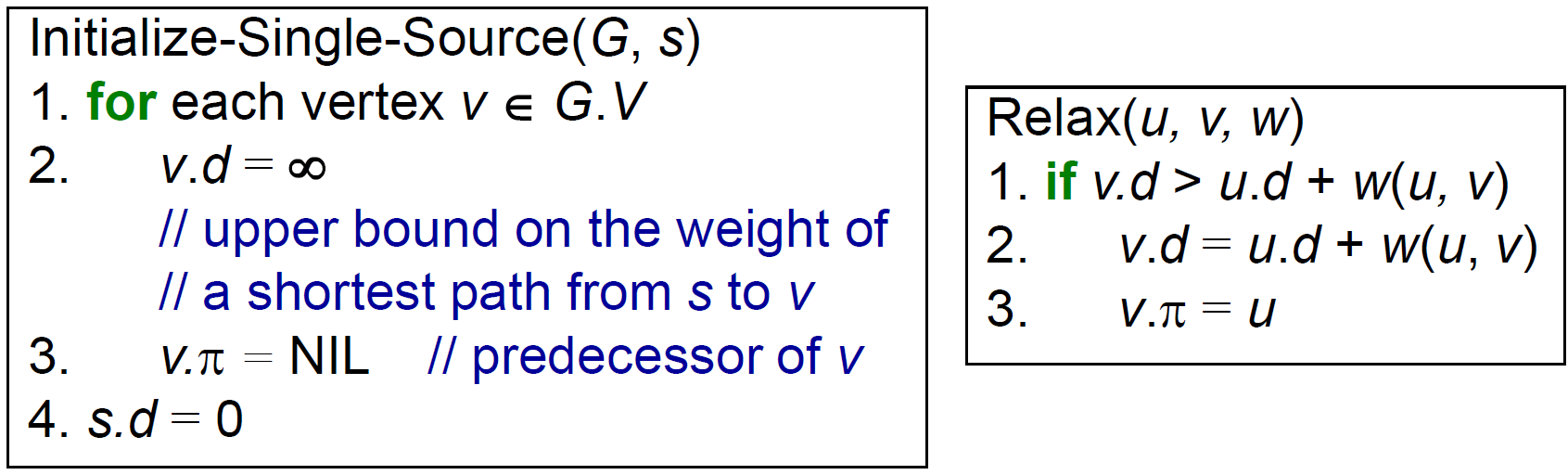
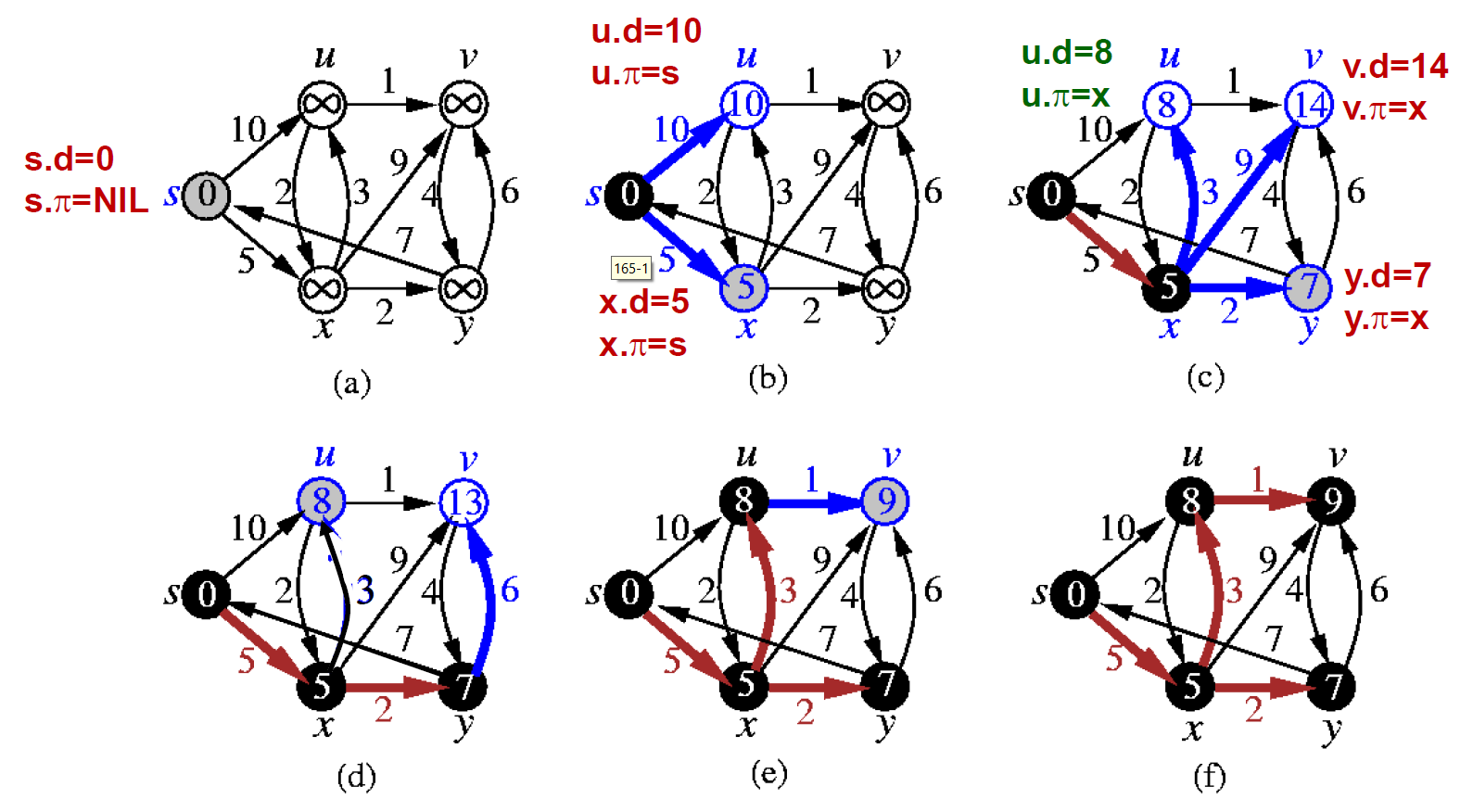
Dijkstra's Algorithm
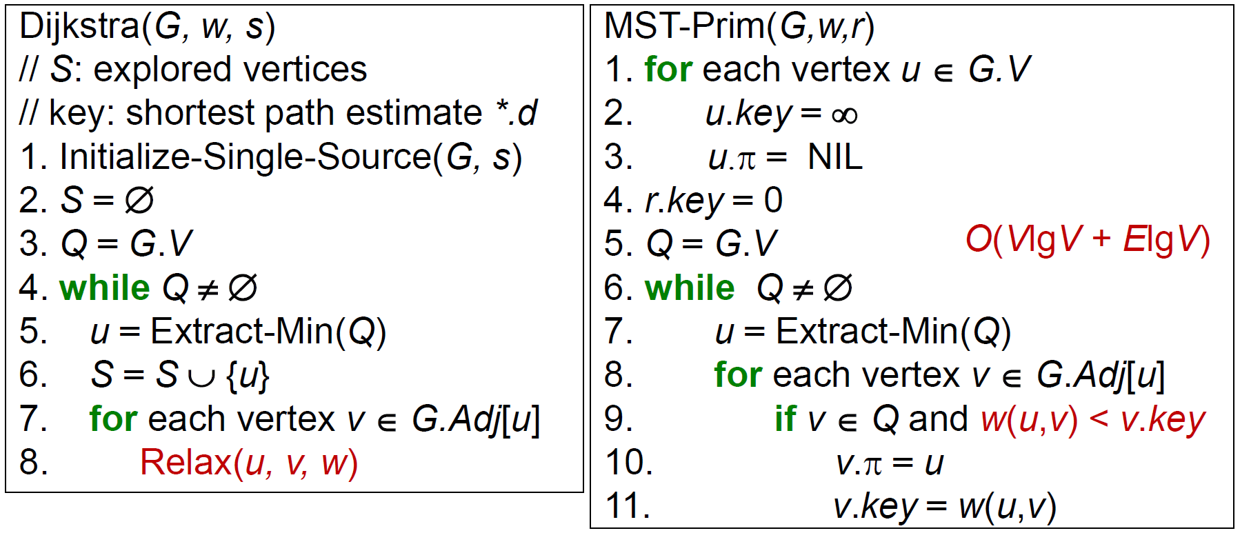
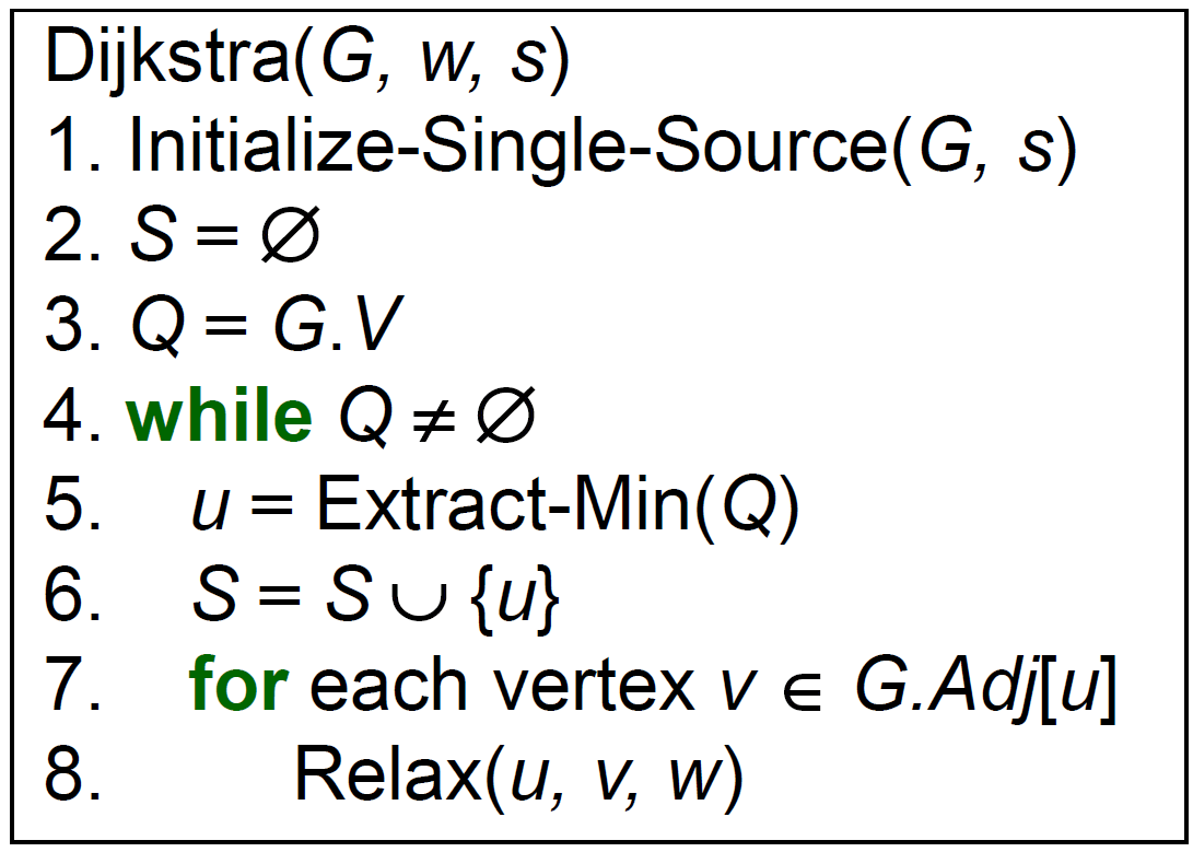
- all edge weights \(\geq 0\)
- Prim's algorithm
- time complexity
- Q = linear array → \(O(V^2)\)
- Q = binary heap → \(O(VlgV)\)
- Q = fibonacci heap → \(O(E+VlgV)\)
- e.g.
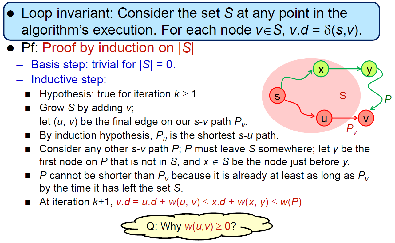
- correctness (?)
- 不接受 negative edges,因為有 nagative edge 則現在找到的 min path might not be min path
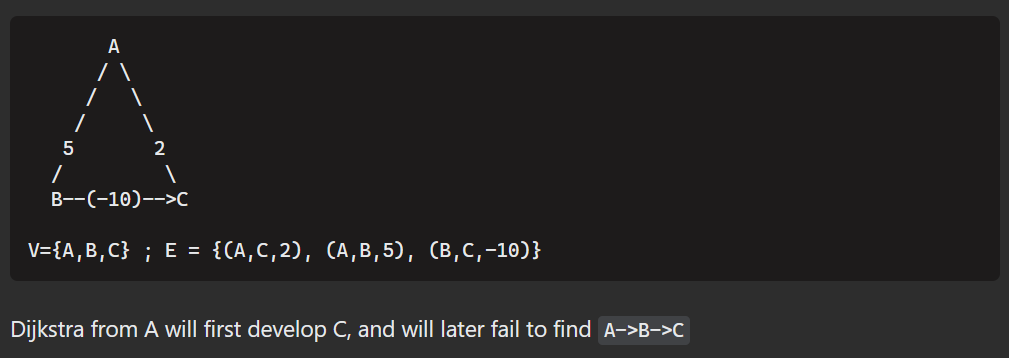
- solution: #Johnson's Algorithm
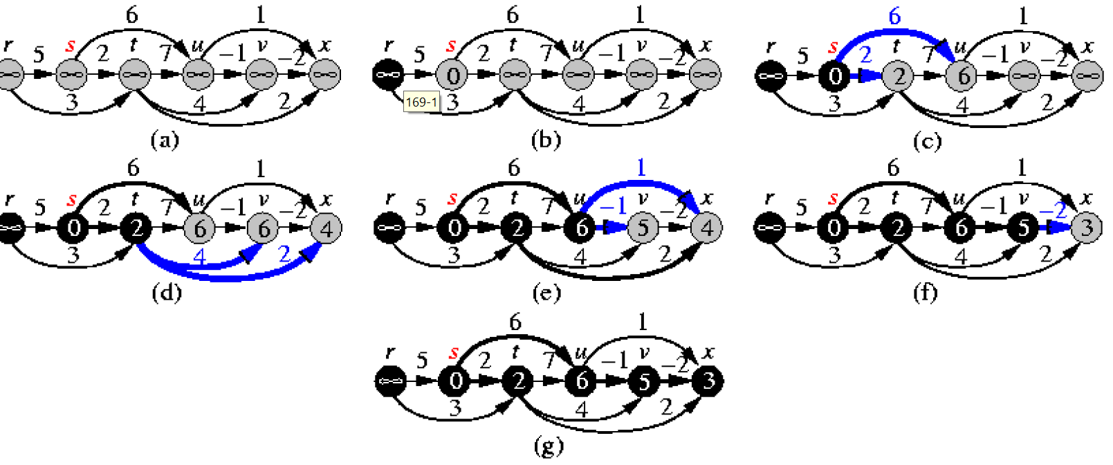
in DAGs
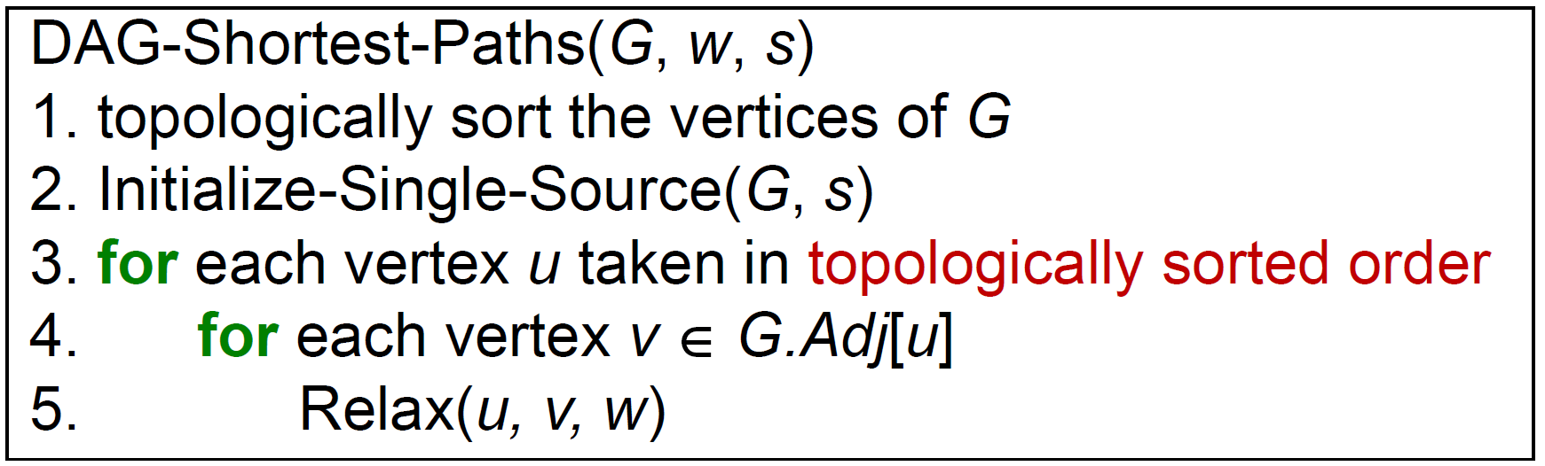
- time complexity \(\in O(V+E)\)
- e.g.
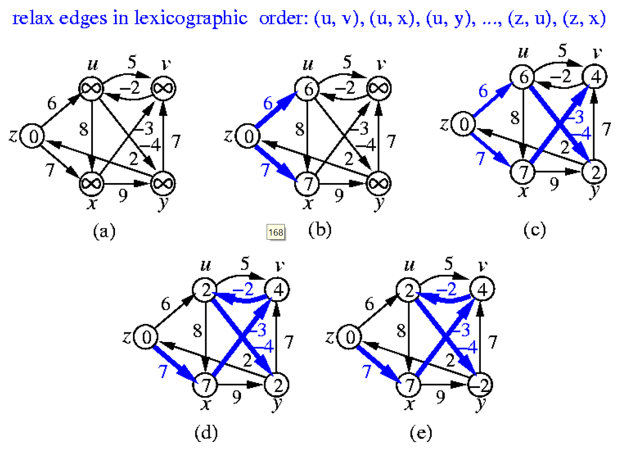
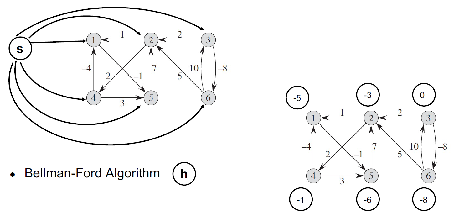
Bellman-Ford Algorithm
def bellman_ford(graph, src):
    # graph format: {"node1", [("node2", 10)]}
    dist = {node: float('inf') for node in graph}
    dist[src] = 0

    n = len(graph)
    for _ in range(n - 1): # at most n-1 edge from src to dst
        for n1, (n2, weight) in graph.items():
            dist[n2] = min(dist[n2], dist[n1] + weight)

    # detect negative cycles
    for n1, (n2, weight) in graph.items():
        if dist[n1] + weight < distances[n2]:
            raise ValueError("Graph contains a negative-weight cycle")

    return distances
- 接受 negative weight edge
- detect negative cycle
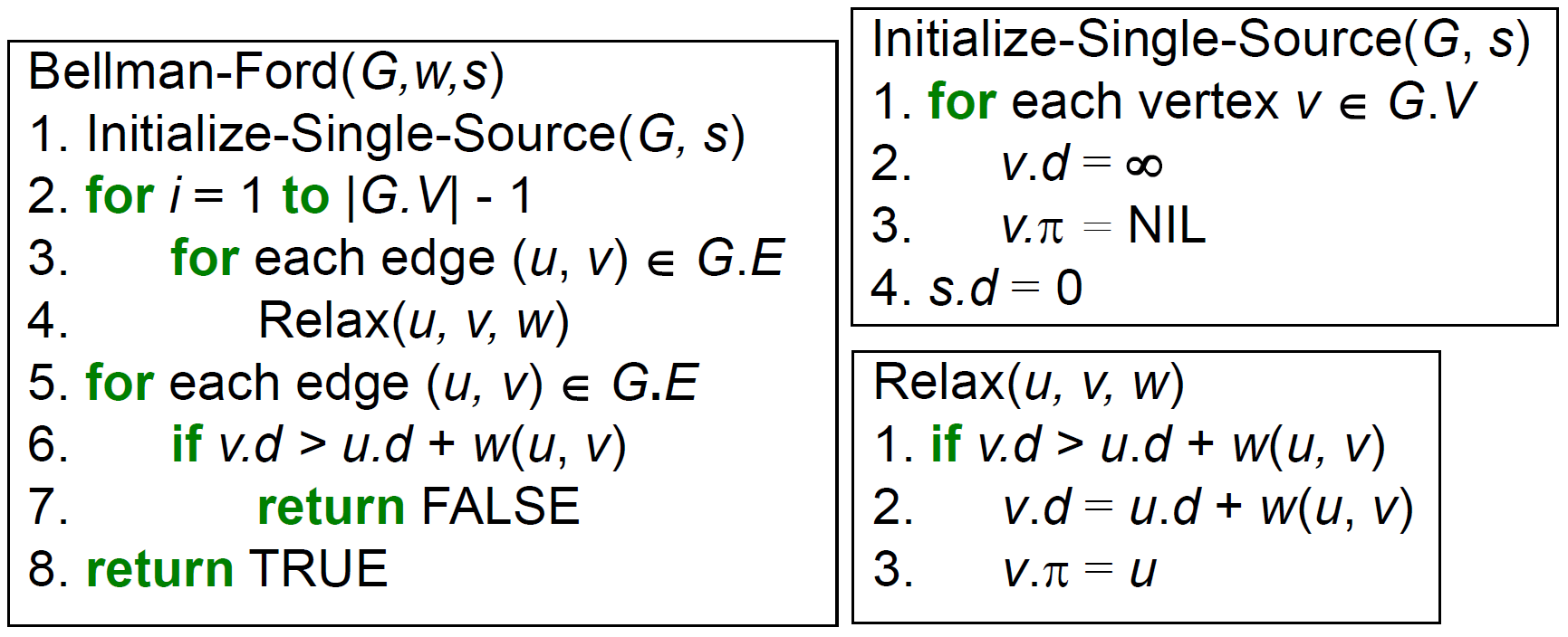
- 5.-7. - if detect negative cycle then return False
- time complexity \(\in O(VE)\)
- e.g.
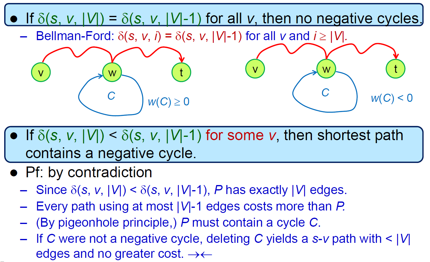
- correction
- negative cycle detection
- bellman-ford 做完後,多 run 一個 iteration 數值會下降 → 有 negative cycle
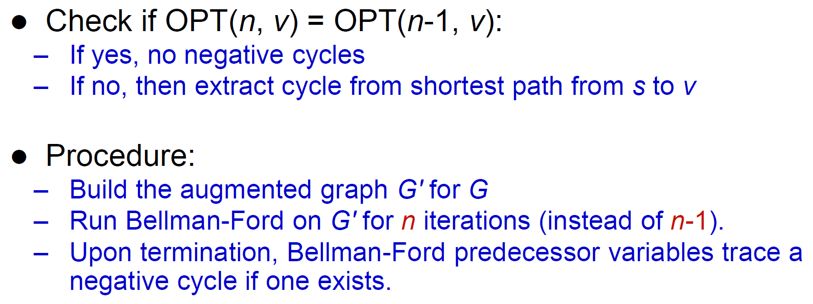
- find negative cycle for a graph
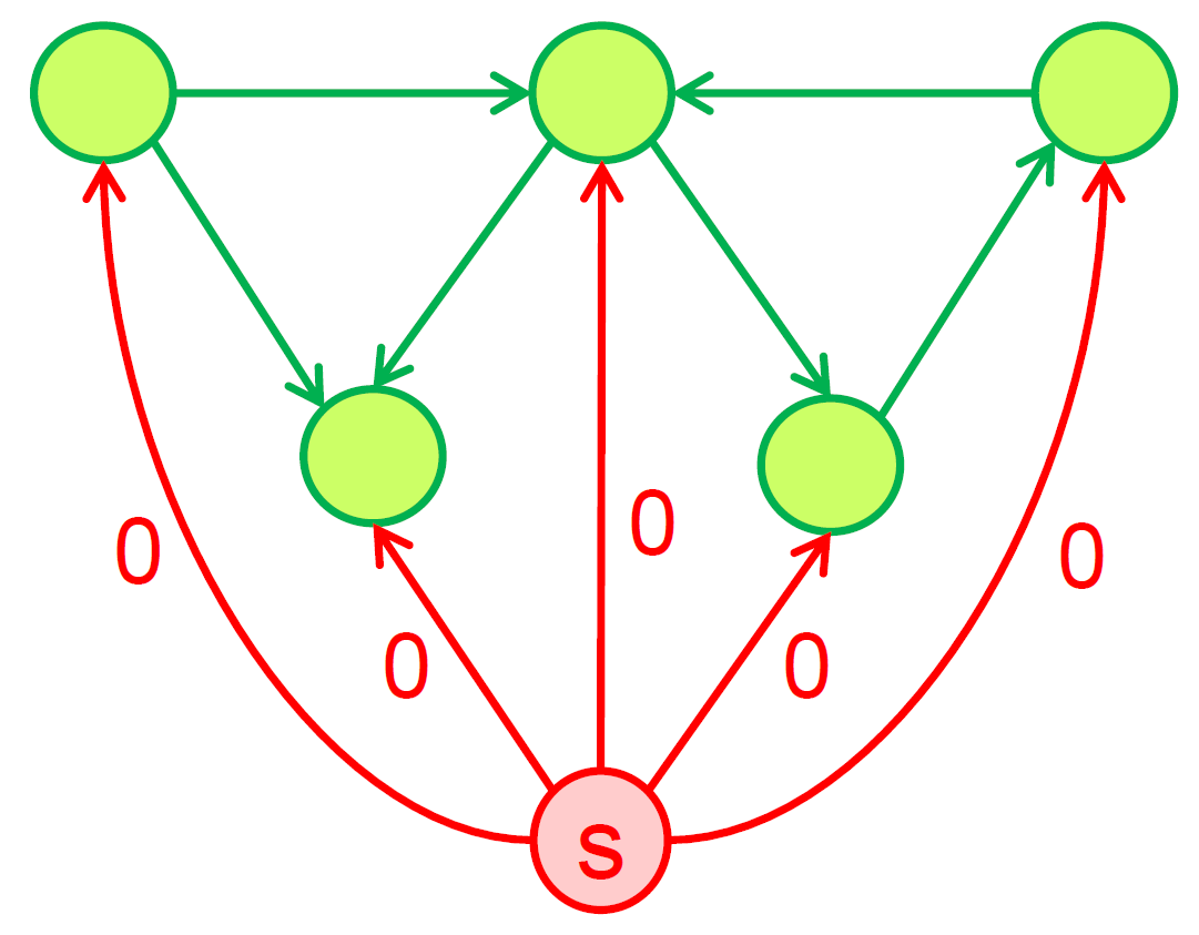
- 做一個 new source S 連到所有 node with 0-cost edge,原本 graph 存在 negative cycle iff 從 S 開始 bellman-ford 找得到 negative cycle
- ?? 為什麼不要直接在原本的 graph 做 bellman-ford ??
- linear programming
- 線性規劃
- constraint graph
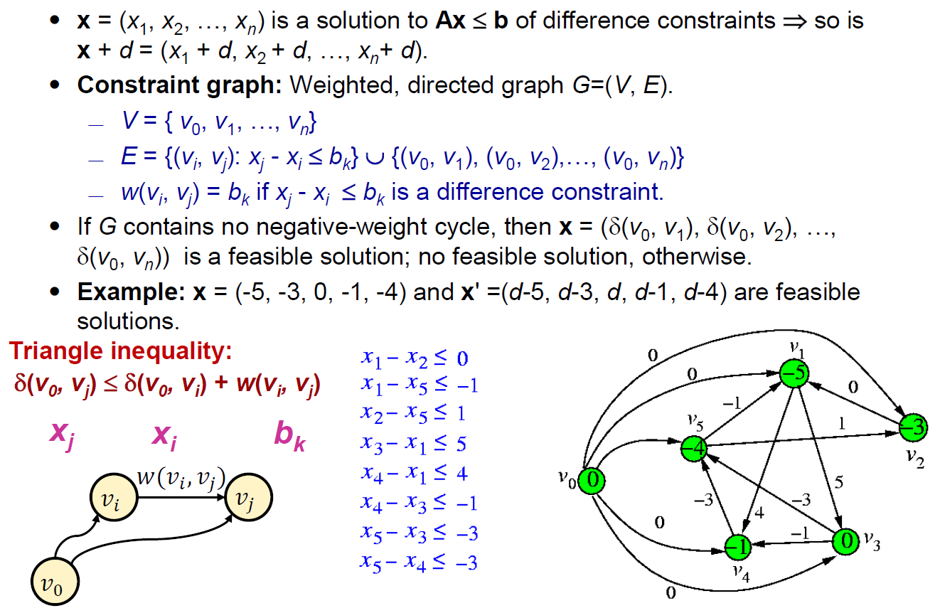
- ???
APSP
- all-pairs shortest paths
- use adjacency matrix
- most use adjacency list
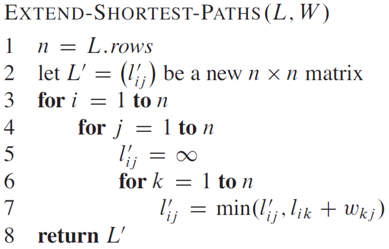
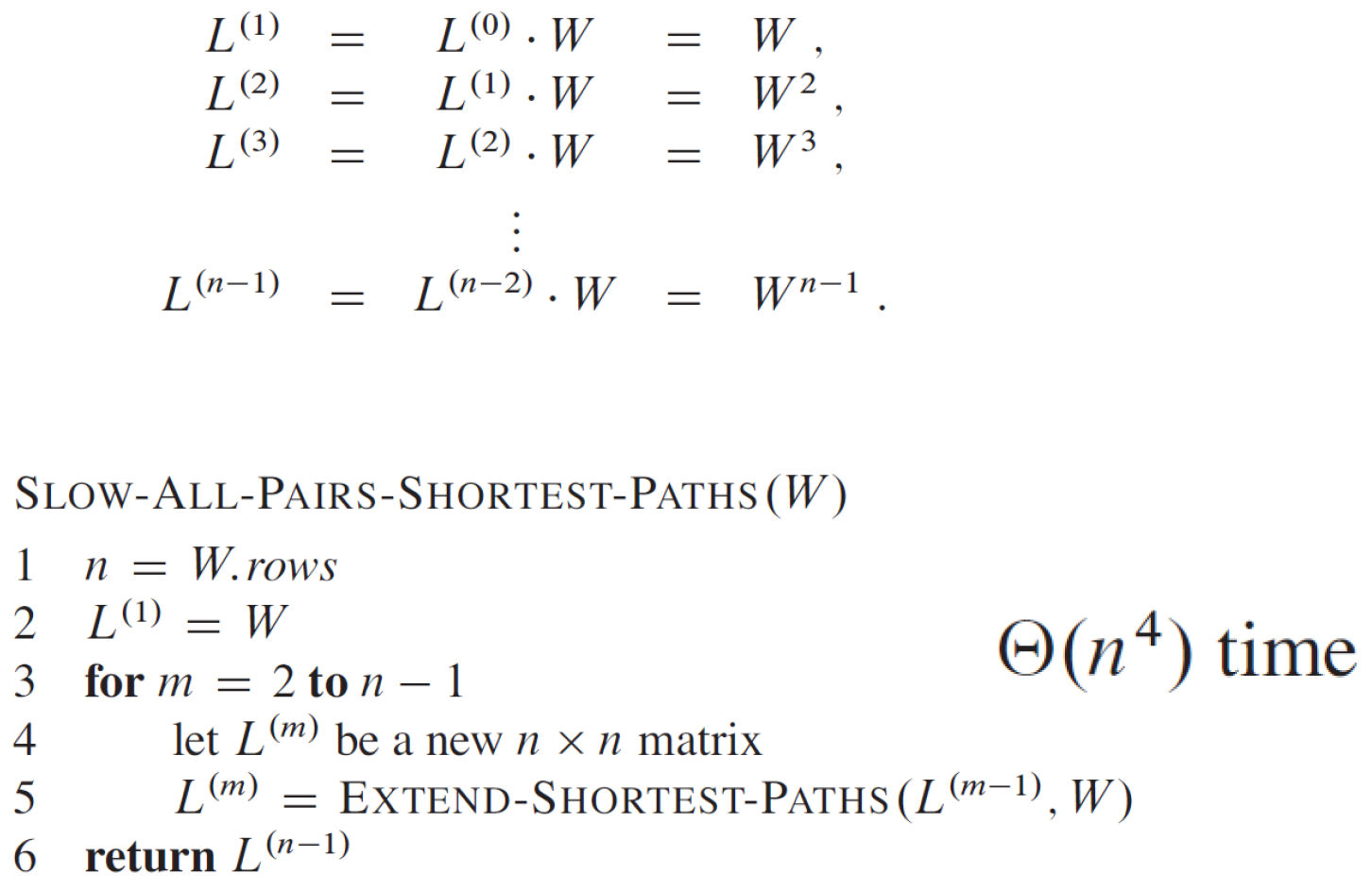
- extened shortest paths
- show all-pairs shortest path
- for \(n^2\) 個 entries,算所有可能的 k 到所有可能的 m → \(\in O(n^4)\)
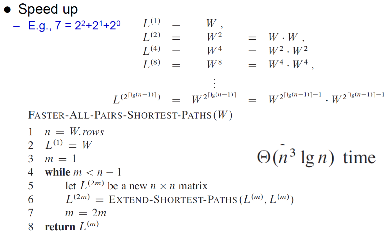
- 可優化
- for \(n^2\) 個 entries,算所有可能的 k 到所有可能的 m → \(\in O(n^4)\)
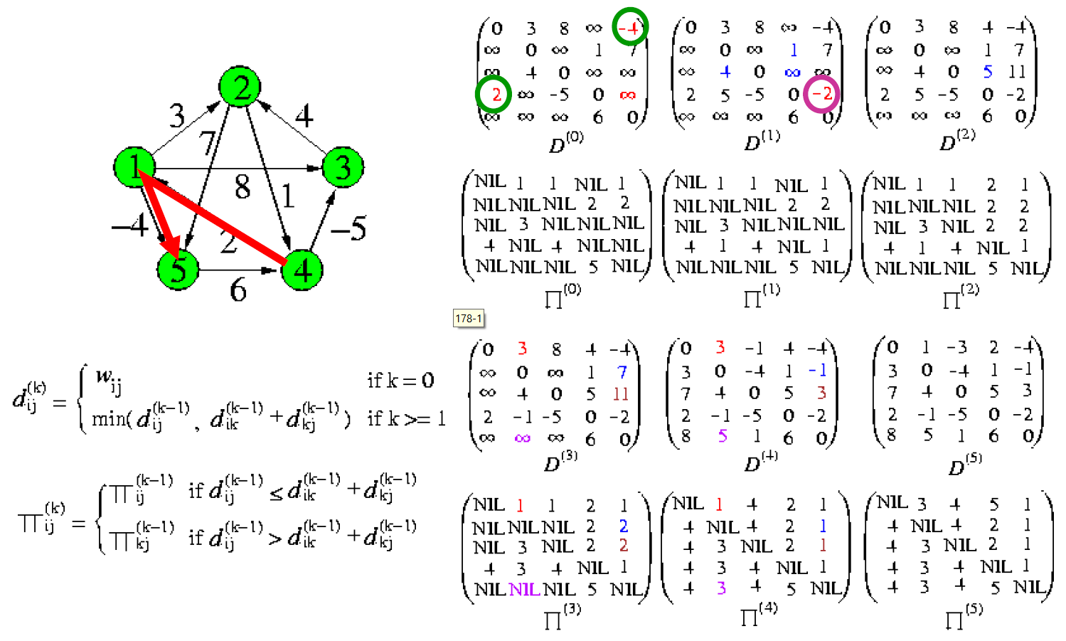
Floyd-Warshell's APSP Algorithm
- i to j subproblem to i to k + k to j
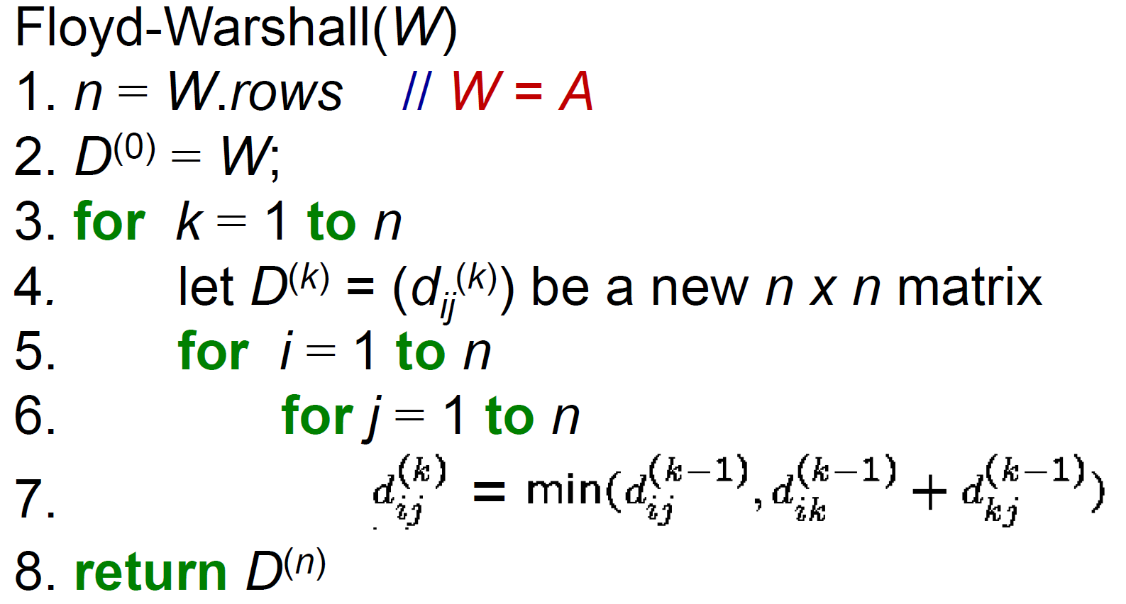
- k 為中繼點
- time complexity \(\in O(V^3)\)
- 執行完對角線上有 < 0 數字 → negative cycle
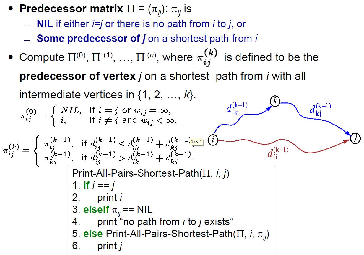
- e.g.
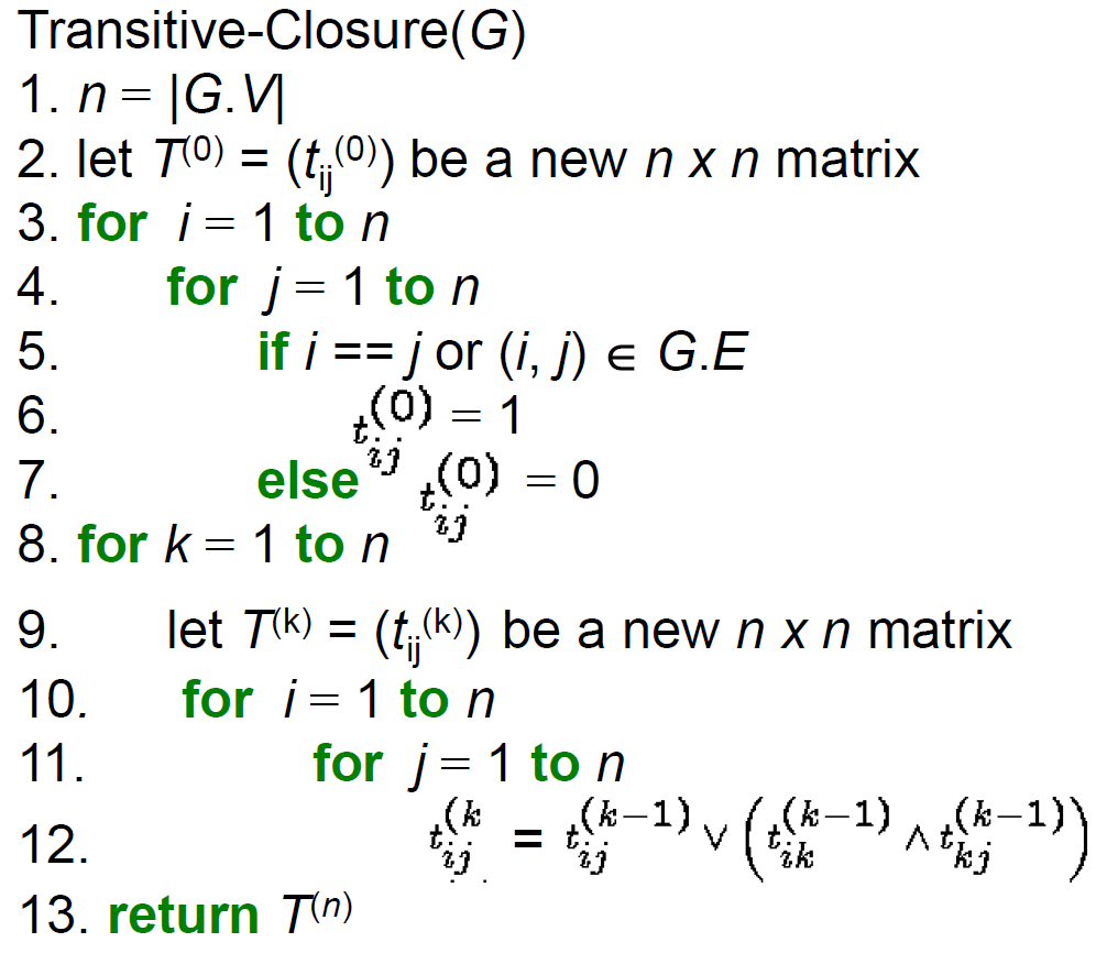
- transitive closure
- i to k AND k to j → i to j
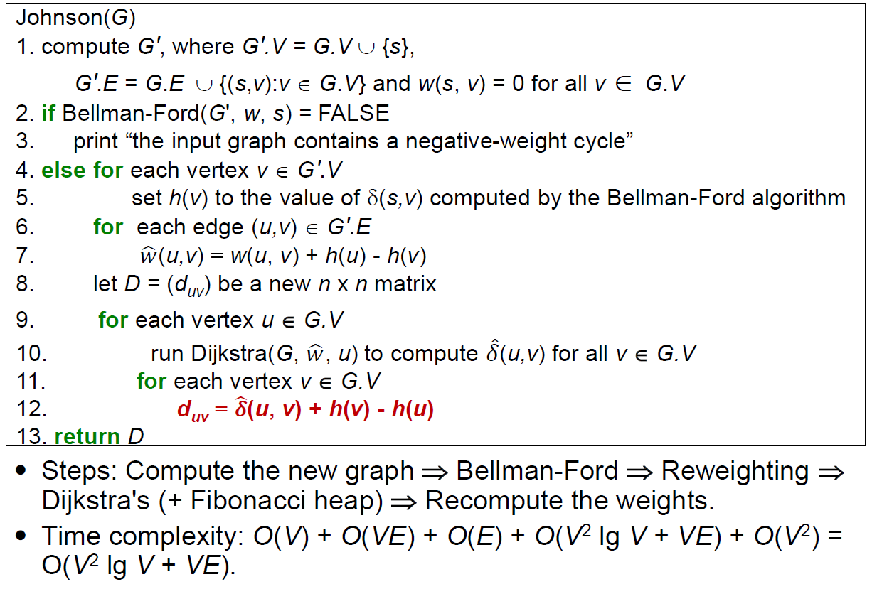
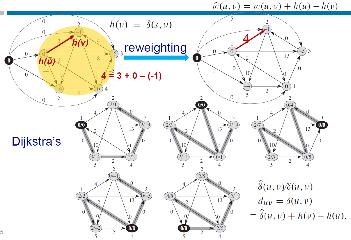
Johnson's Algorithm
- https://www.geeksforgeeks.org/johnsons-algorithm/
- can't have negative cycle (use Bellman-Ford Algorithm to verify)
- reweight s.t. all edges are nonnegative without changing the shortest path solution → Dijkstra's Algorithm
- 移動 node 的位置
- \(h(u)\) = 把 node u 往前移動多少
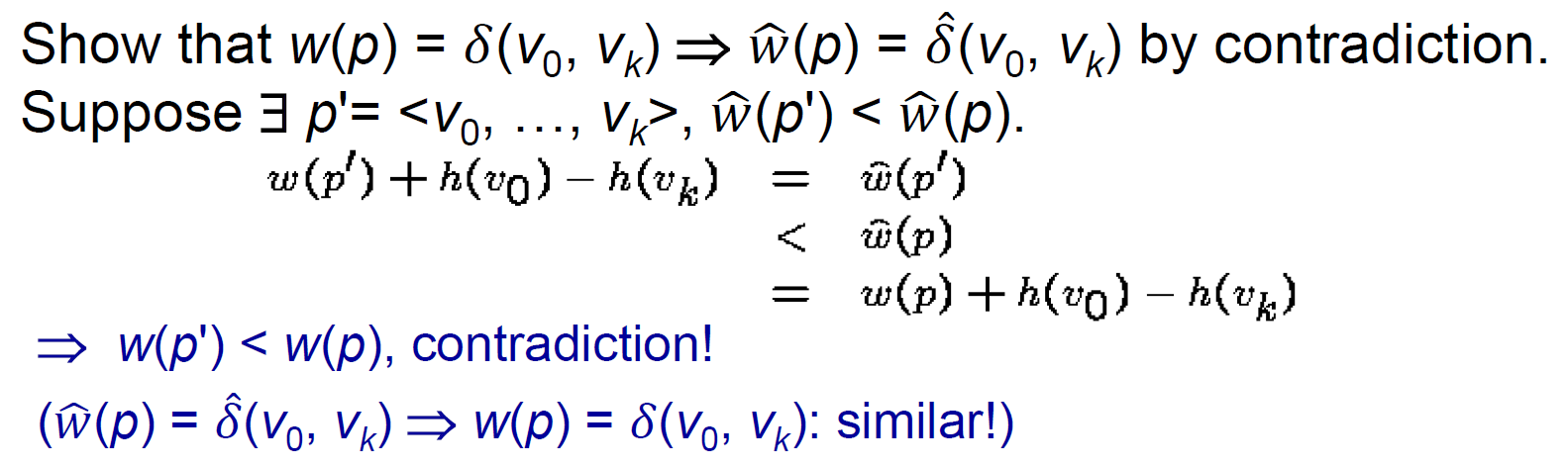
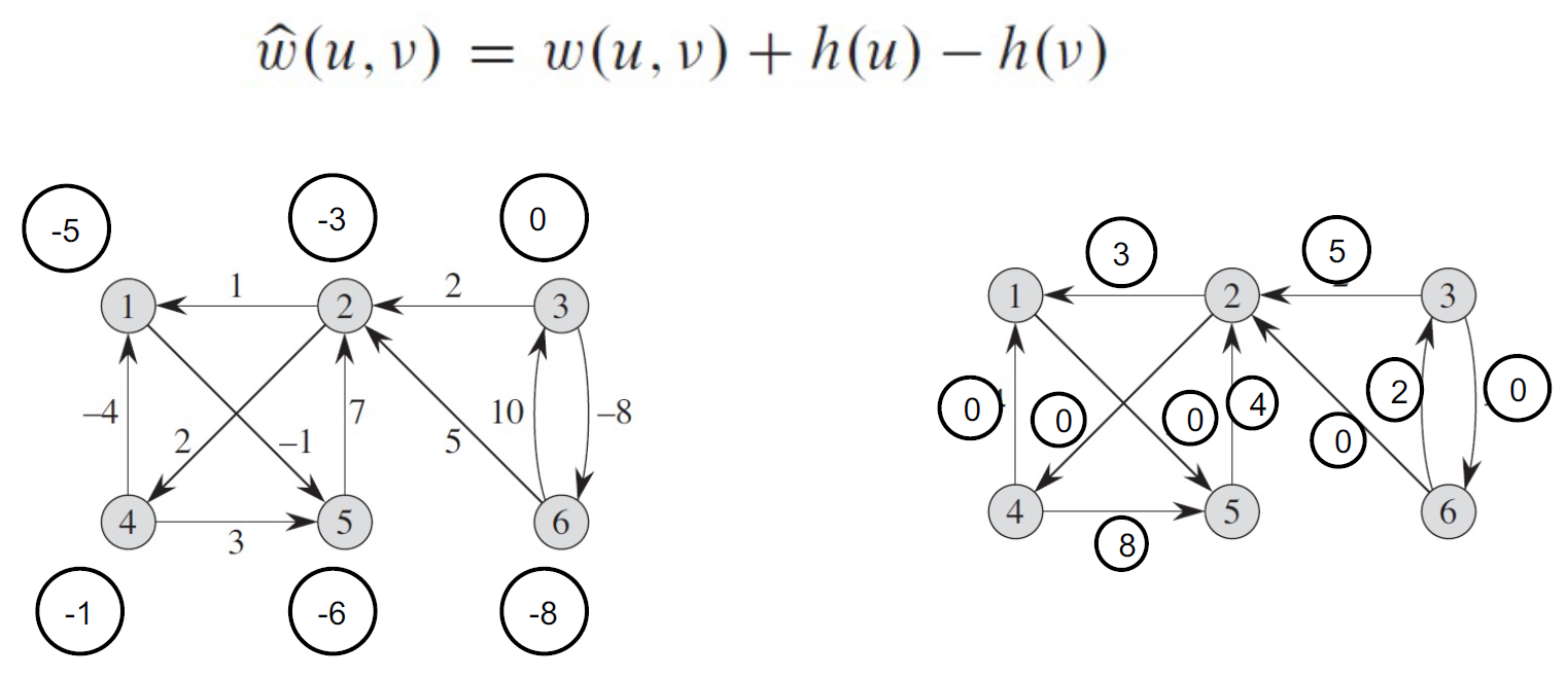
- \(\hat{w}(u,v)=w(u,v)+h(u)-h(v)\)
- 經過很多點,各點會互相 cancel,只留起終點的淨移動量,so 兩點間的每個 path 改變相同,shortest path 不變
- shortest path 不變
- create new node connecting to every node with edge weight 0,shortest distance → h i.e. node 移動的量
- e.g. h(u) = -3, h(v) = -5 → w(u,v) -= -2
- cycle preserving
- cycle 位置都跟原本一樣
- e.g.
- yellow: 原本 graph
- create new node 接上所有 node with weight 0
- run Bellman-Ford Algorithm
- red edge 的起點提前 0,終點提前 -1 → new weight = 3+1 = 4
- 下面是 node 表示法:altered cost / 反推回的 original cost
Flow Network
- directed graph
- 求 max flow
- e.g.
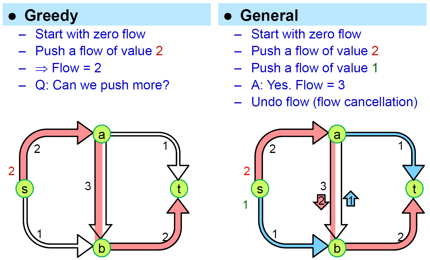
- s → a → b 後,推 1 回 a → t ,其餘 2 繼續 b → t
- flow out = flow in
- augmentating path = 可灌更多 flow 的 path
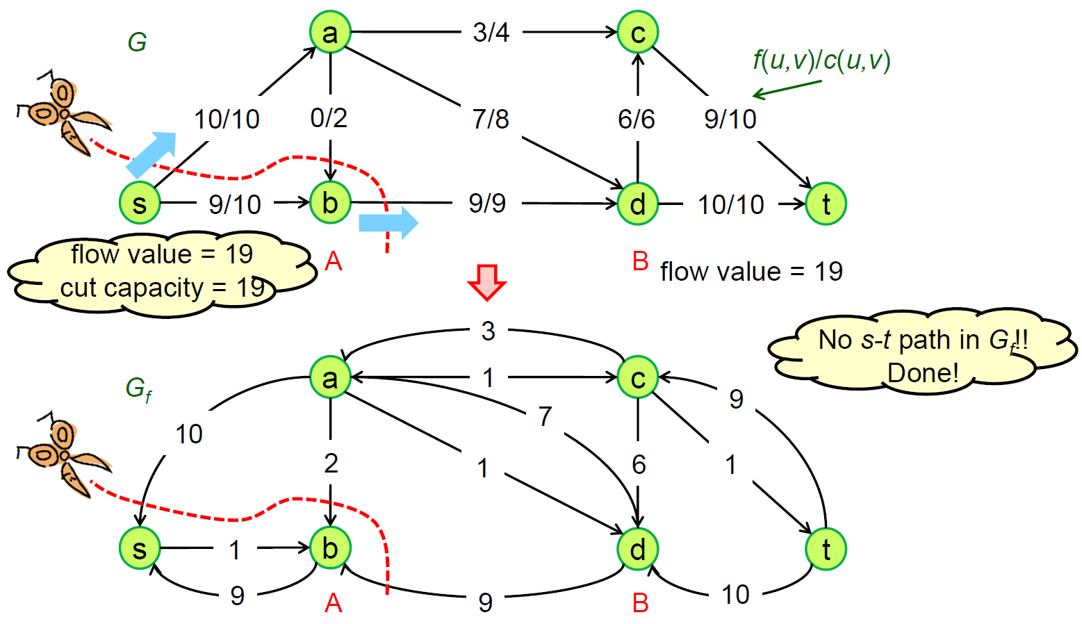
max-flow min-cut theorem
- https://brilliant.org/wiki/max-flow-min-cut-algorithm/
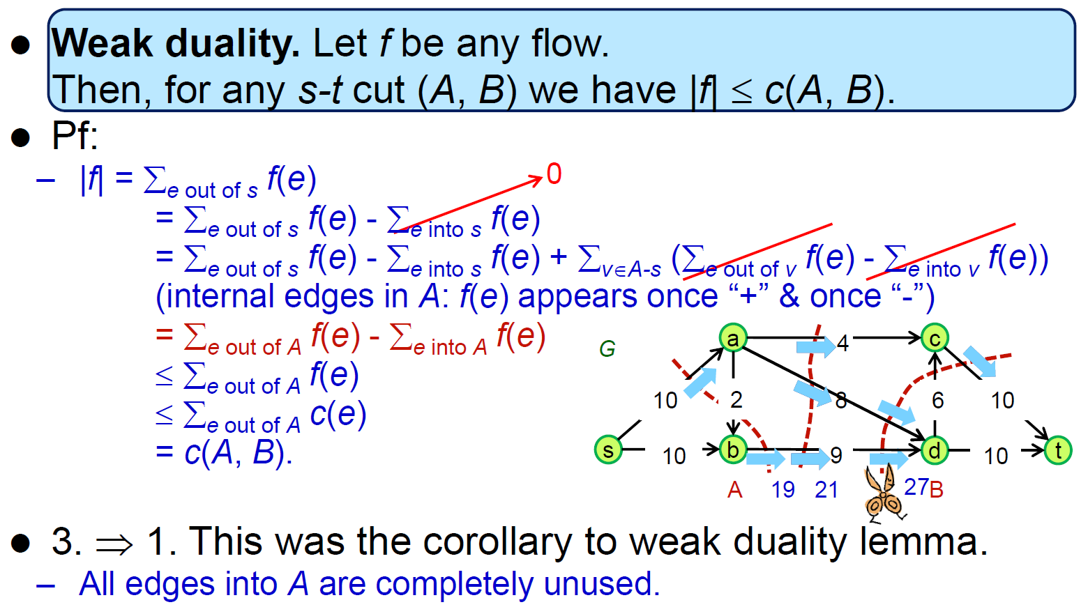
- 每個 cut 都是一個 upper bound → min cut is the min upper bound i.e. the real upper bound
- 只算 toward destination 的 edge
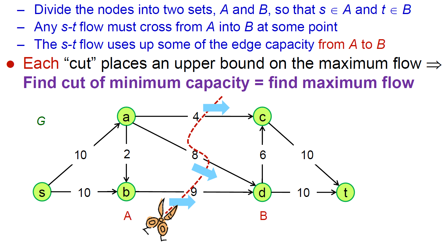

- proof
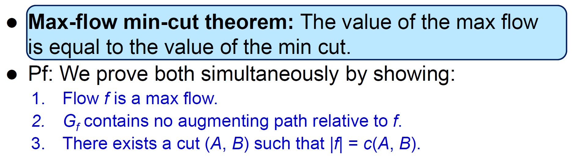

- 有 augmentation path → 可以灌更多 → not max flow
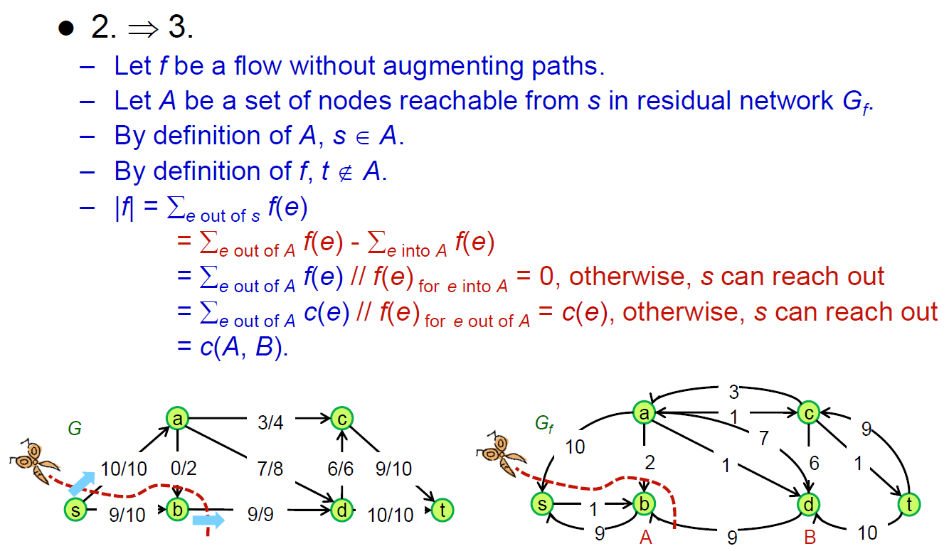
- 一定會用盡 capacity,否則還會有路出去
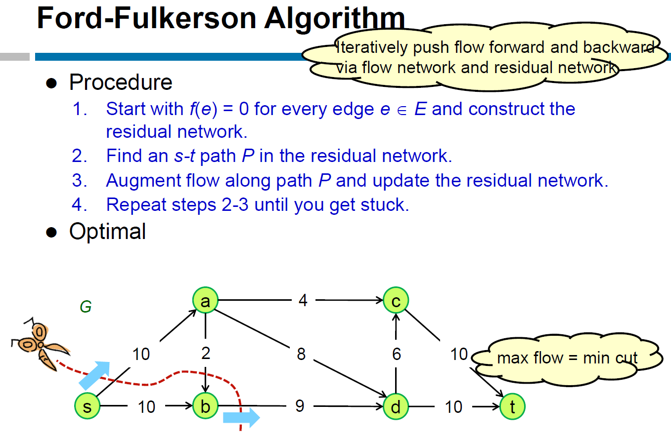
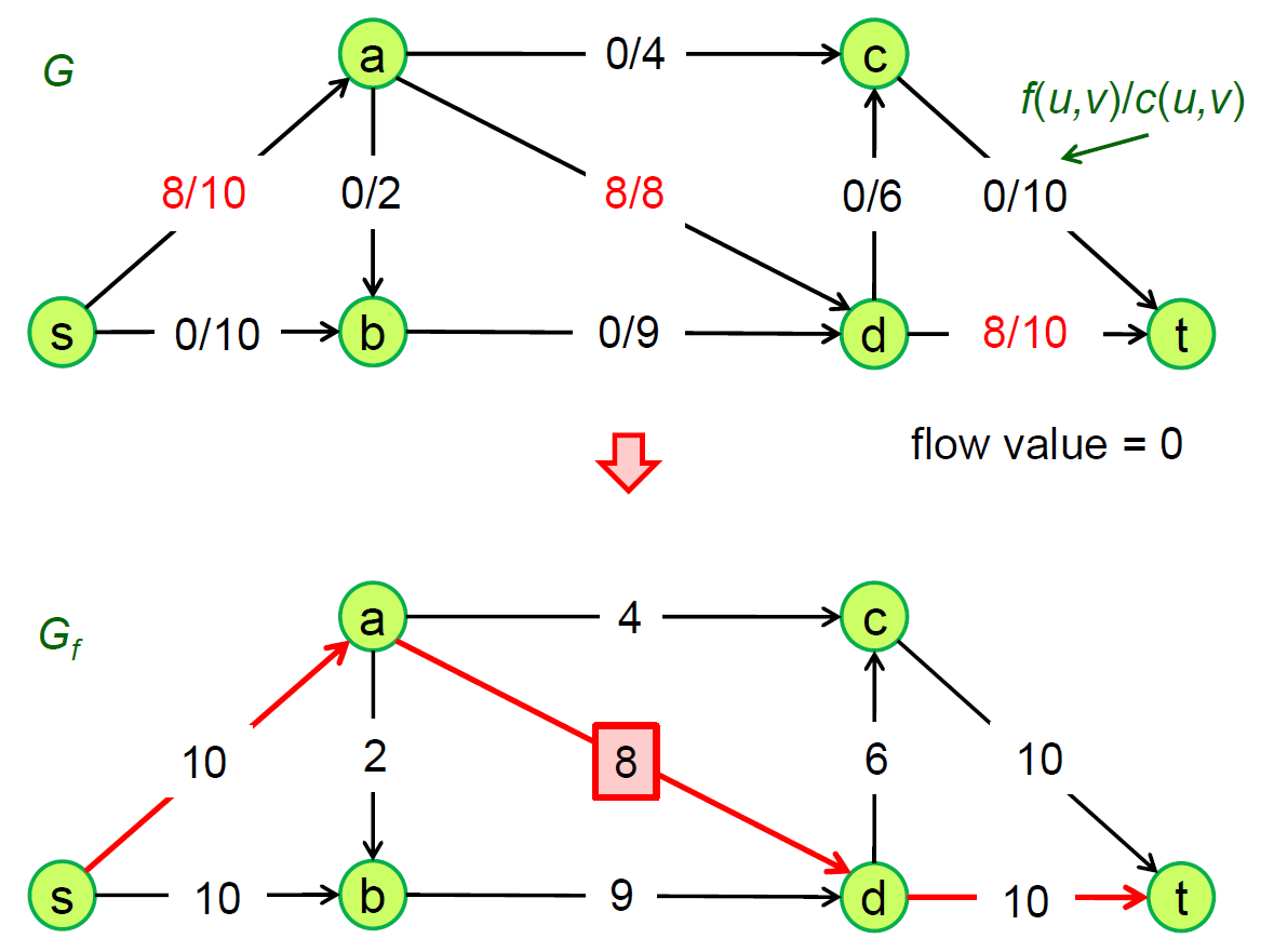
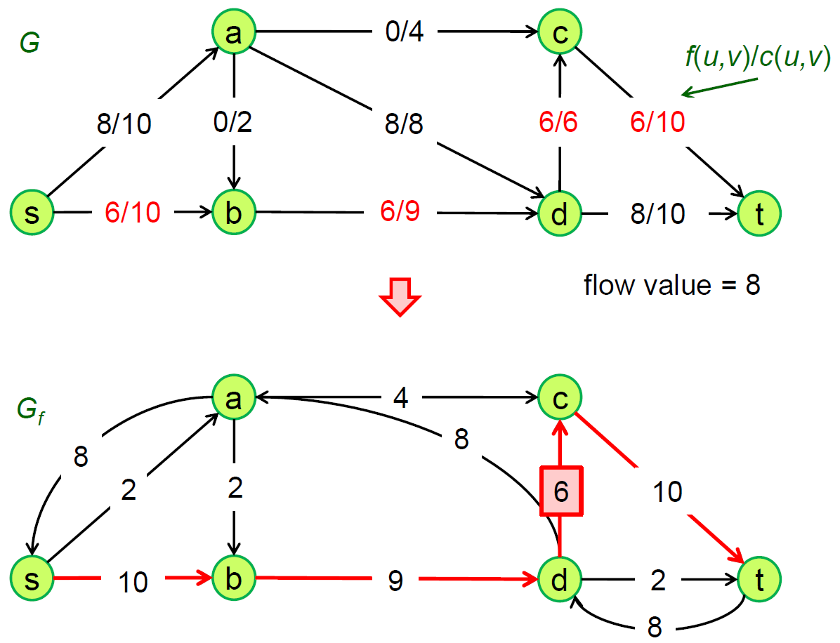
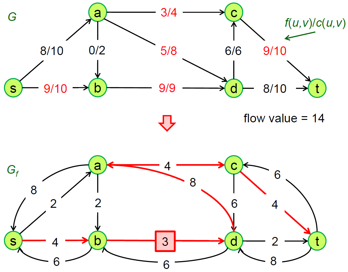
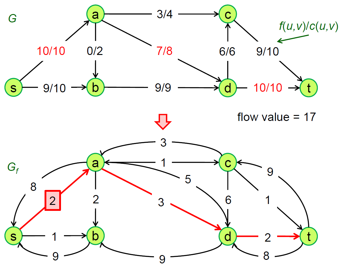
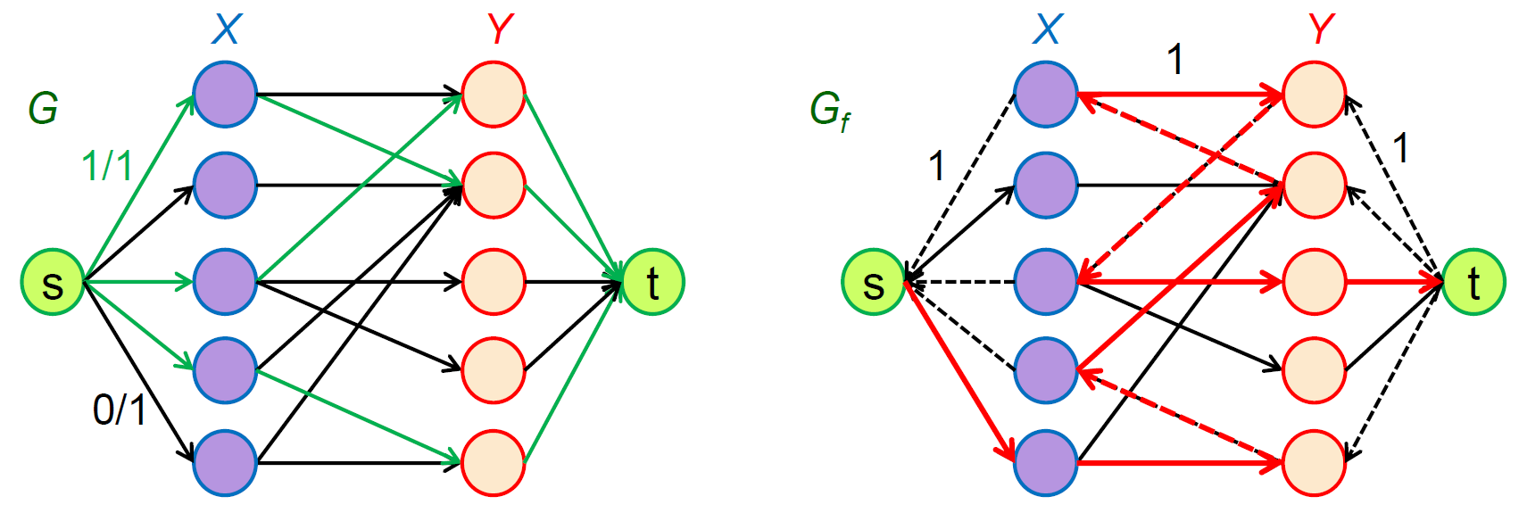
Ford-Fulkerson Algorithm
- residual network
- 在 flow network,s to t 找到 path → 更新 flow network 各 edge 的 capacity,更新 residual network,把 path 都弄成 backward edge → repeat
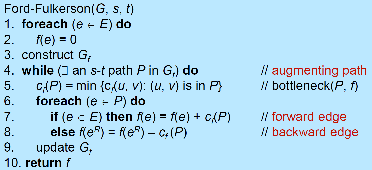
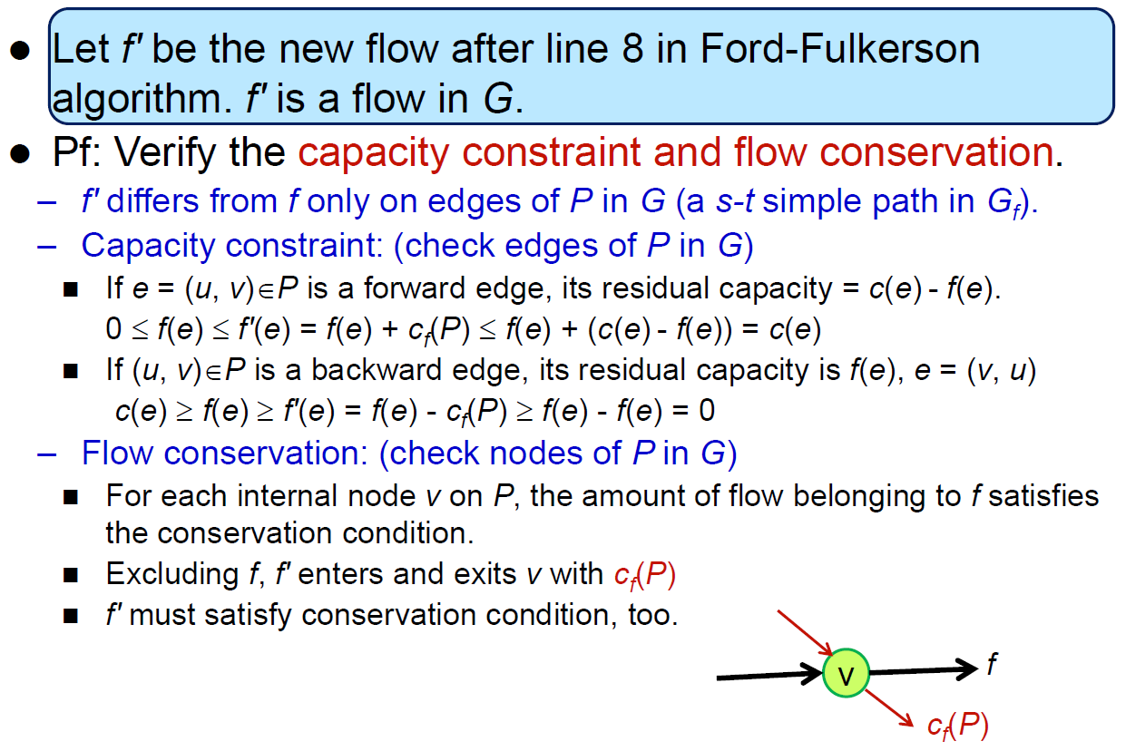
- legal flow pf
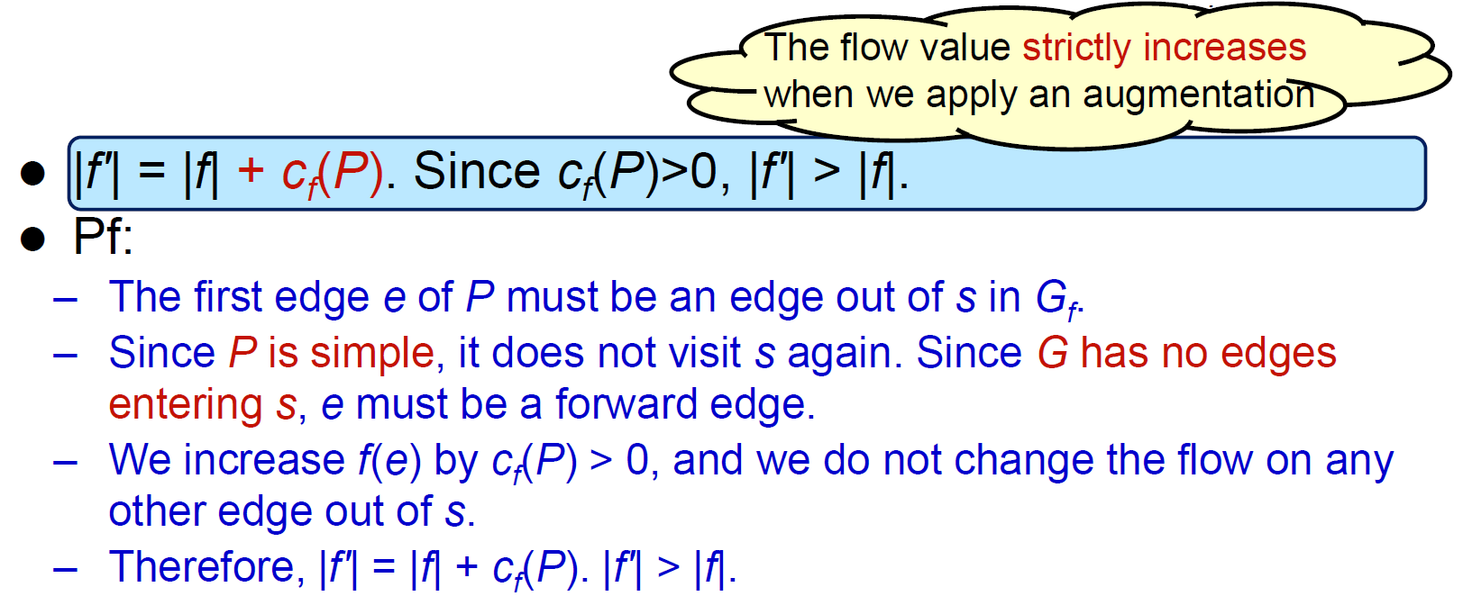
- flow will increase after applying augmentation
- time complexity \(\in O(EC)\)
- not polynomial to input size (but capacity)
- at most C iterations
- C = flow upper bound
- each aumentation increase flow by at least 1 → at most C iterations

- e.g.

- worst case 200 interations
- each augmentation \(O(V+2E)=O(E)\)
- e.g.
Edmonds-Karp Algorithm
- https://brilliant.org/wiki/edmonds-karp-algorithm/
- #Ford-Fulkerson Algorithm but find the shortest augmentation path (min edges) in residual network with BFS
- time complexity \(\in O(VE(V+E))=O(VE^2)\)
- \(\dfrac{VE}{2}\) iterations
- an edge is critical when it's filled → edge reversed
- distance from source would increase at least 2 at the next time it become critical
- max distance = V → max iteration = V/2 for each node
- \(V+E\) each iteration (path finding)
- BFS
- \(\dfrac{VE}{2}\) iterations
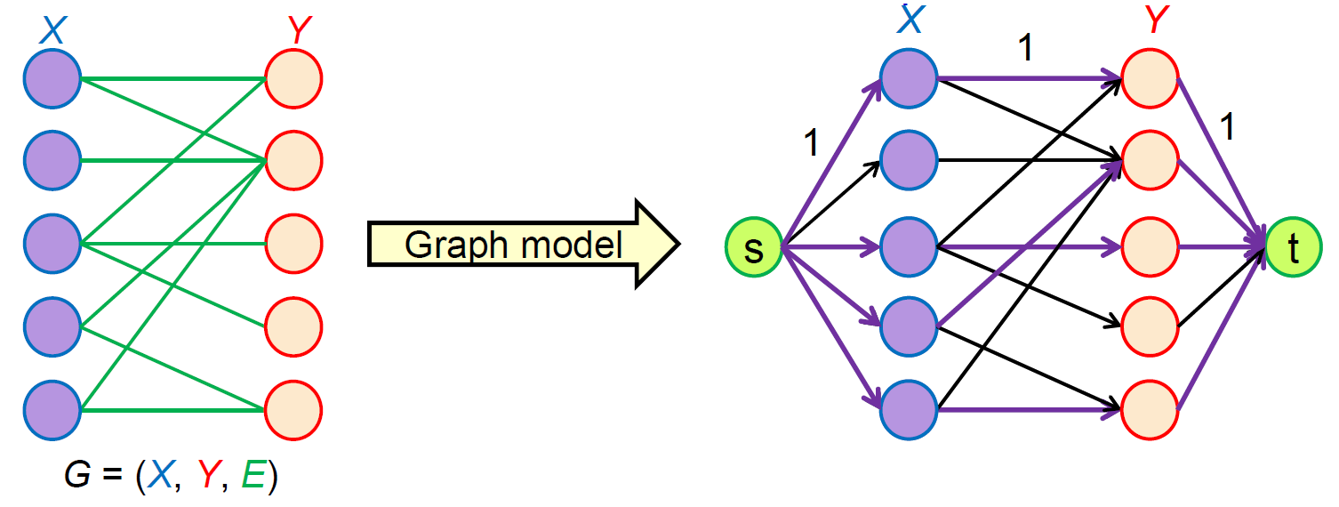
Bipartite Matching
- no 2 edges share same endpoints
- build a flow network and find the max flow
- only 1 direction
- create source & destination
- each edge's capacity = 1
NP-completeness
decision problem
- output True/False
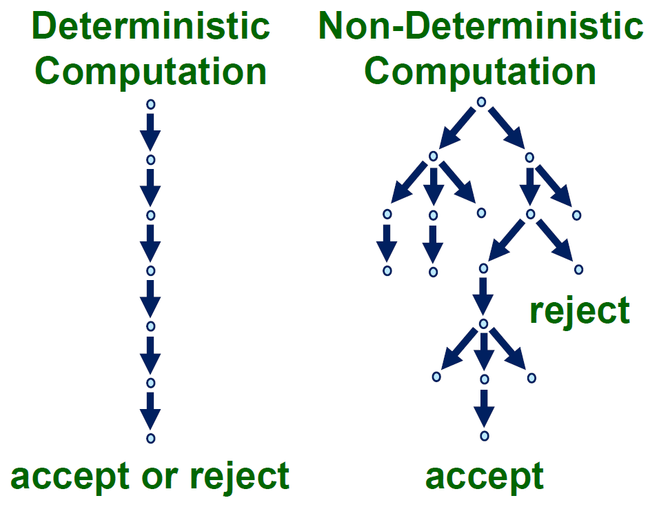
turing machine
- DTM, deterministic turing machine
- 1 outgoing edge
- NTP, nondeterministic turing machine
- multiple outgoing edges
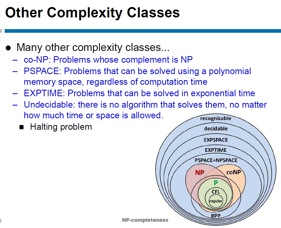
class P
- polynomial-time solvable
class NP
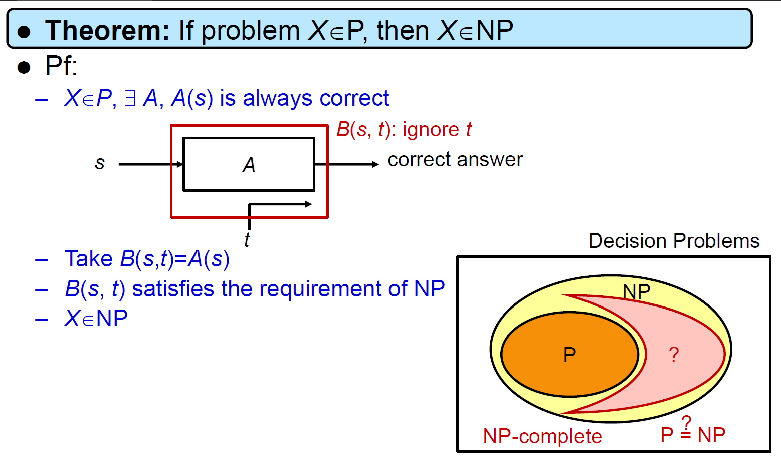
- polynomial-time verifiable by NTM
- for decision problem
- \(P\in NP\)
- e.g.
- set cover problem
- Are there k subsets of set U s.t. their union is U?
- procedure (polynomial-time)
- for each subset, if an element of U isn't presented, indicate with 0, otherwise 1
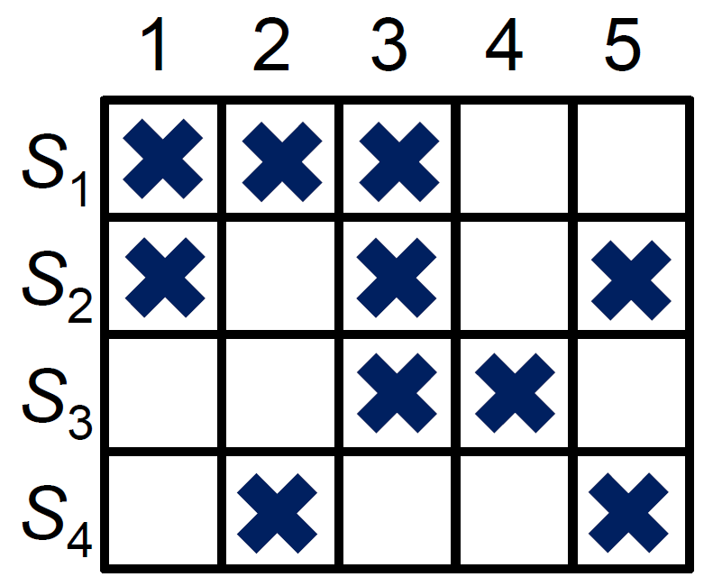
- set cover problem
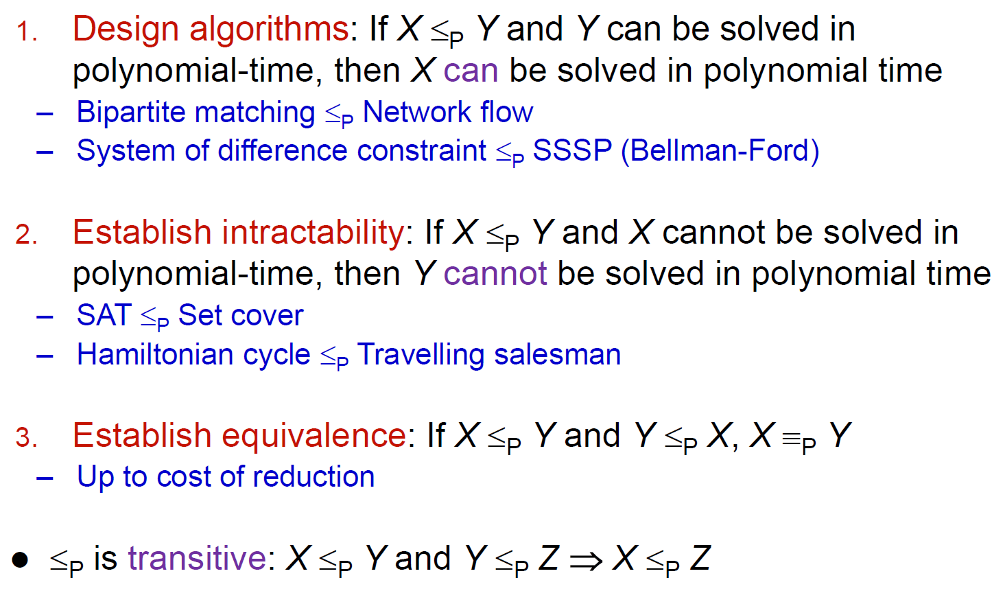
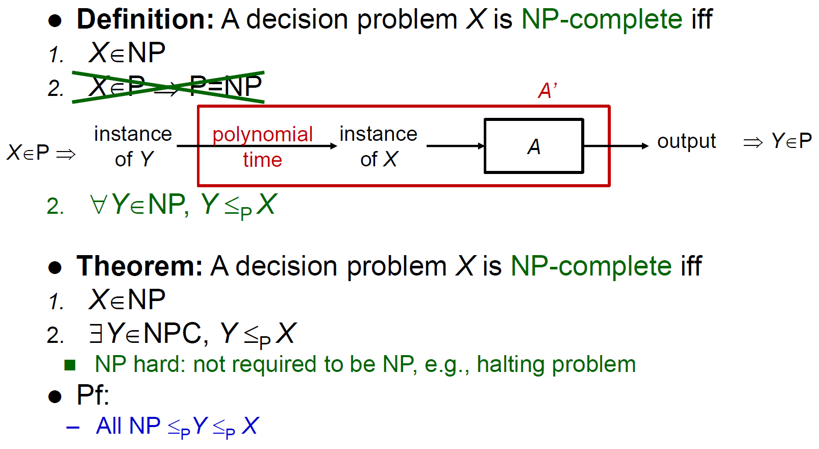
polynomial-time reduction
- algo A can solve Y, then we'll do some mapping in polynomial-time and solve X with A
- \(X\leq_P Y\) (polynomial-time reduction function f from X to Y)
- f(x)=y \(\in Y\) for any x
- x is true iff f(x)=y is true
- mapping function is polynomial-time
- hardness of Y >= X
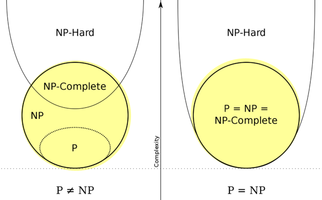
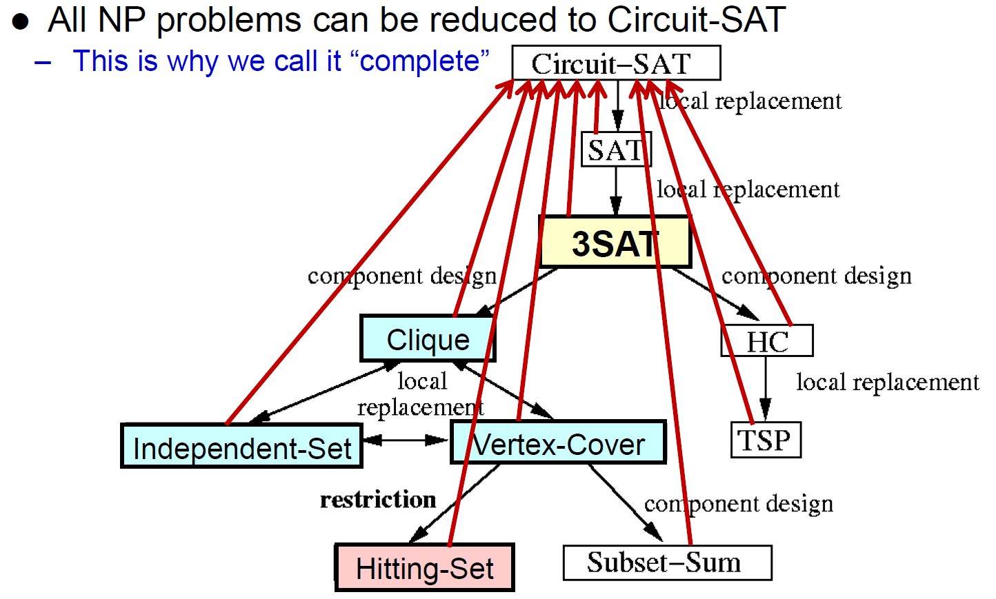
class NP-complete
- hardest problems in NP
- if any NP-complete problem \(\in P\), then \(P=NP\) (???????)
- both NP & NP-Hard
- NP <- 猜一個 答案,可以在 polynomial-time 被驗證
- NP-Hard <- exist an NP-Complete problem that can do polynomial-time reduction into it
- e.g. Hamiltonian path/cycle, set cover, Tetris, Sudoku
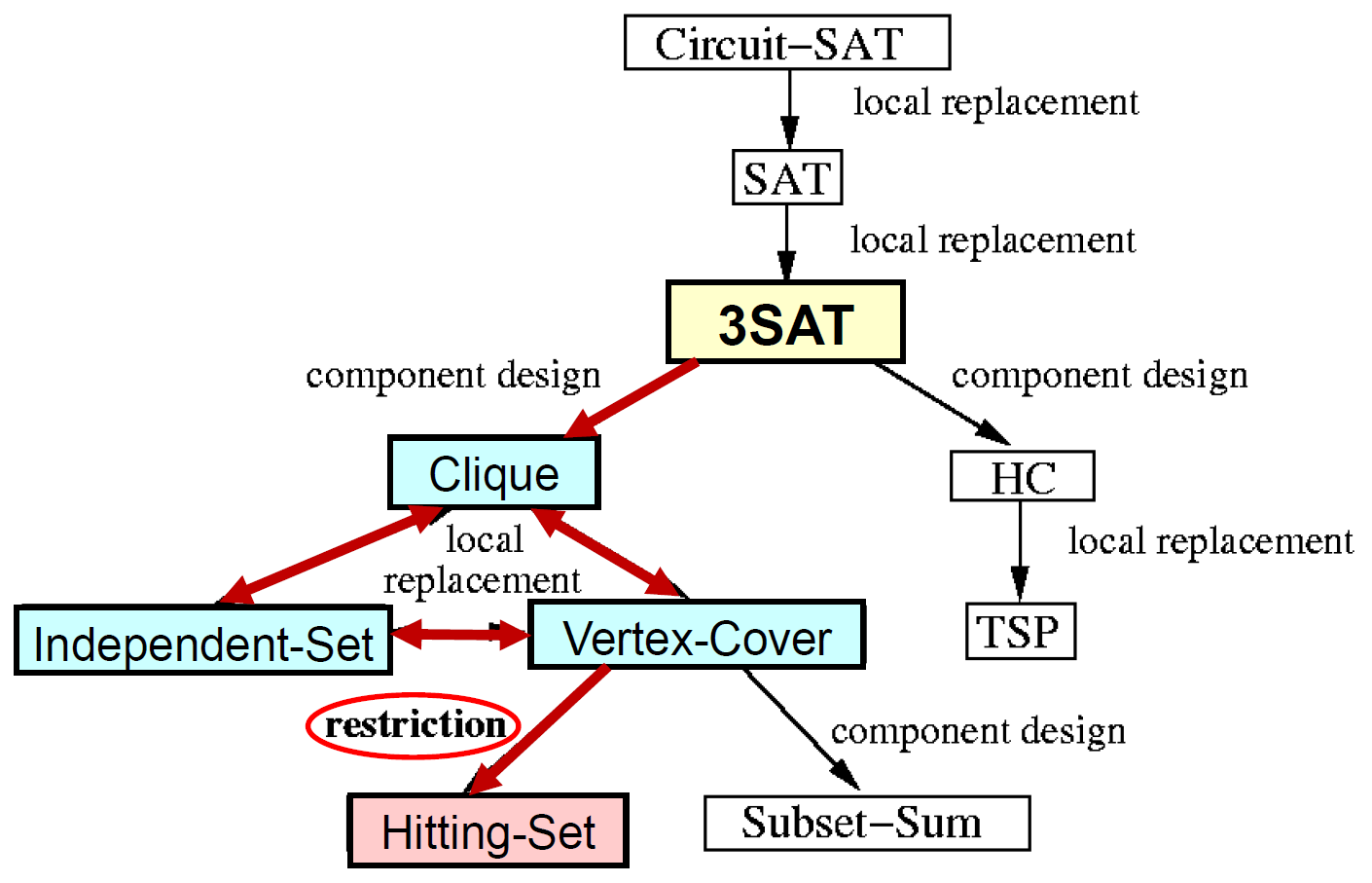
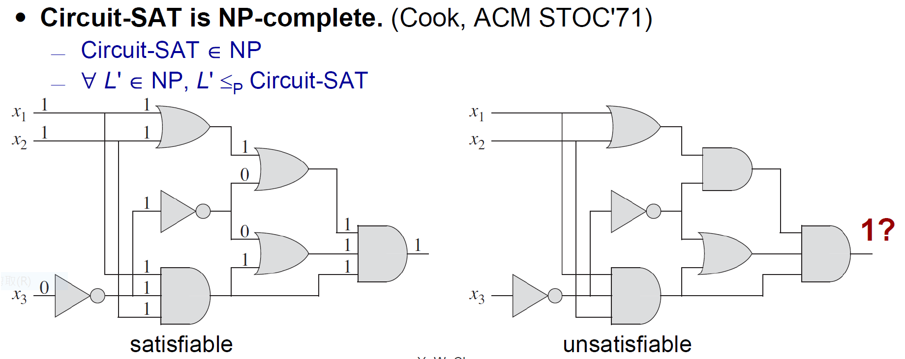
SAT
- Satisfiability Problem
- CNF = conjuntive normal form
- (a+b)x(c+d)
- literal = variable
- clause = (a+b)
- Circuit-SAT \(\in\) NP
- NP-Complete
- SAT \(\in\) NP
- SAT \(\in\) NP-Hard
- bc Circuit-SAT \(\leq_p\) SAT
- set cover
- nSAT = 每個 set 最多 n 個
- 3SAT
- 3SAT \(\in\) NP
- 3SAT \(\in\) NP-Hard
- bc SAT \(\leq_p\) 3SAT
clique
- a subgraph that every 2 distinct elements is adjacent
- clique problem (Clique) \(\in\) NP-Complete
- problem: Is there a clique of size \(\geq\) k ?
- Clique \(\in\) NP
- Clique \(\in\) NP-hard
- 3SAT \(\leq_p\) Clique
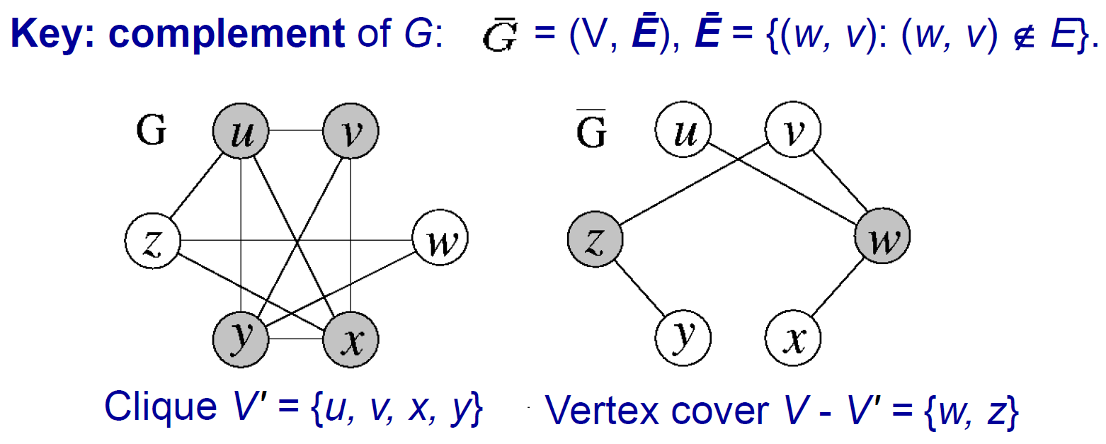
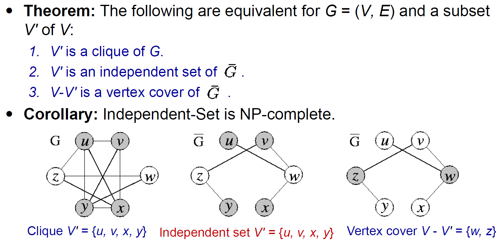
vertex cover
- problem: Is there \(V'\subseteq V\) s.t. every edge has an endpoint in \(V'\)
- vertex cover is a complete subgraph
- vertex cover \(\in\) NP
- vertex cover \(\in\) NP-hard
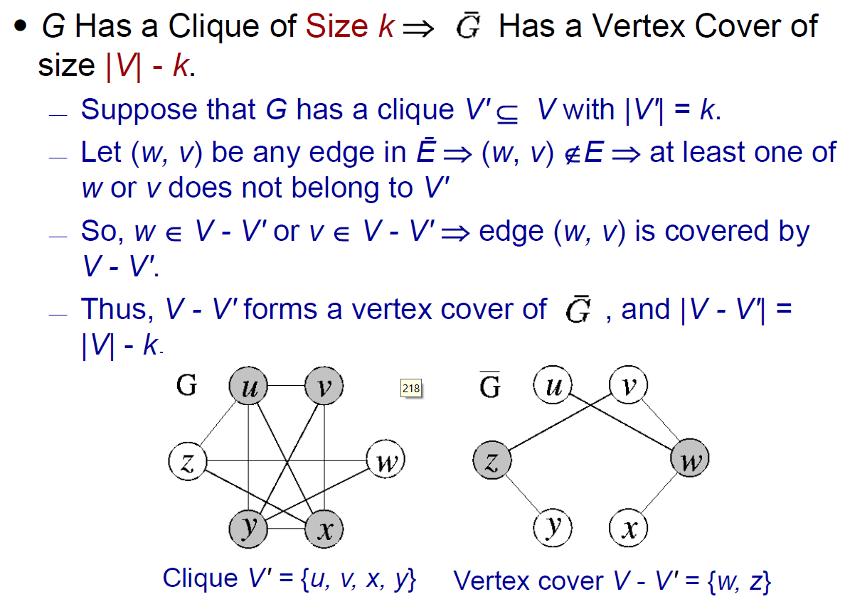
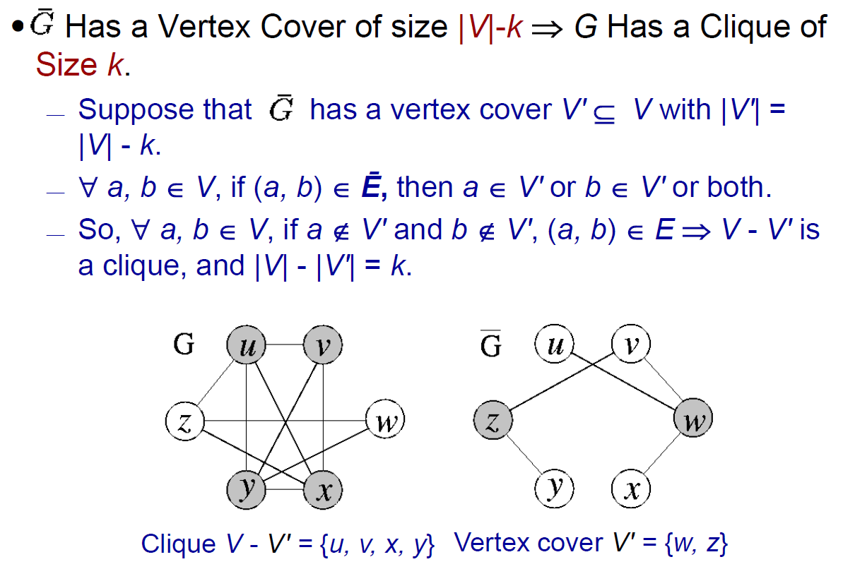
- Clique \(\leq_p\) vertex cover
- 有 clique → 有 vertex cover
- 若有 clique,則剩下的 nodes + 不存在的 edge (\(\bar{E}\)) 就會形成 vertex cover
- 右邊的 edge (\(\bar{E}\)) 至少有 1 個 endpoint 不在 clique 裡面
- 2 個 endpoints 都在 clique → 會是左邊的 edge (E) → 右邊 (\(\bar{E}\)) 不會有這條 edge
- 右邊的 edge (\(\bar{E}\)) 至少有 1 個 endpoint 不在 clique 裡面
- 若有 clique,則剩下的 nodes + 不存在的 edge (\(\bar{E}\)) 就會形成 vertex cover
- 有 vertex cover → 有 clique
- 有 clique → 有 vertex cover
- Clique \(\leq_p\) vertex cover
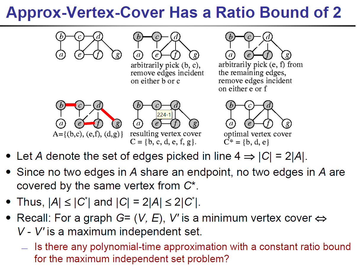
- approx vertex cover algo
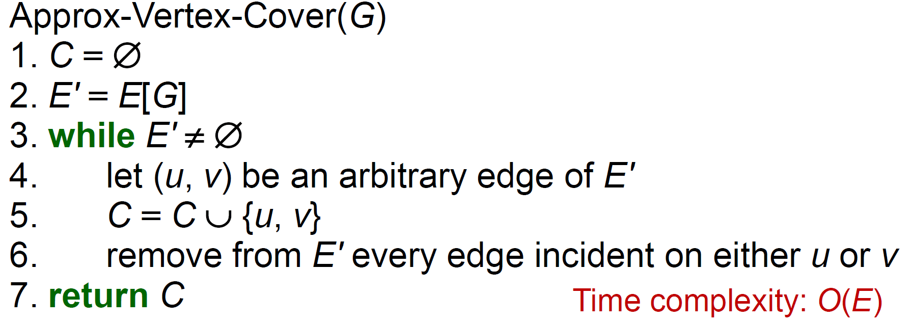
- 找到的解會是最佳解的兩倍以內
- e.g.
- 得到 {b,c,e,f,d,g},but 最佳解是 {a,c,f,g}
- 3SAT → vertex cover
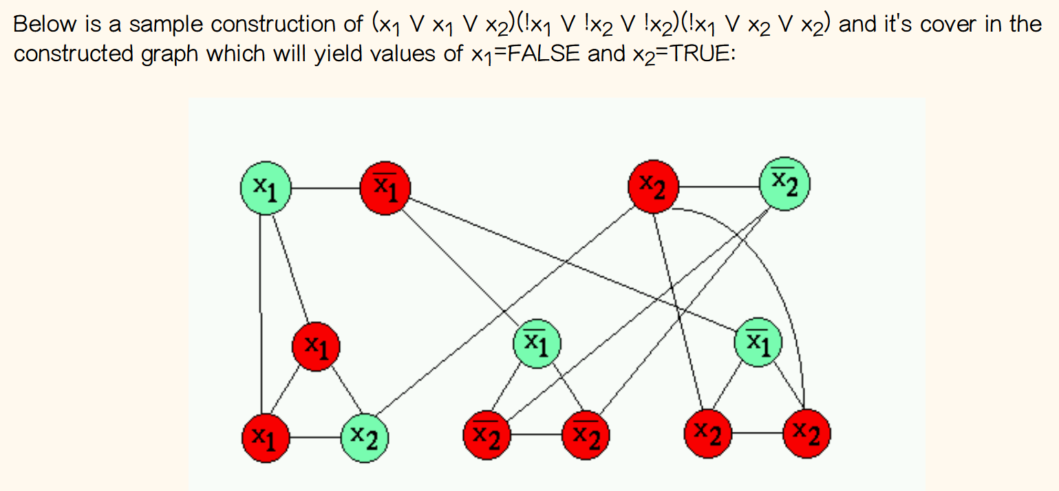
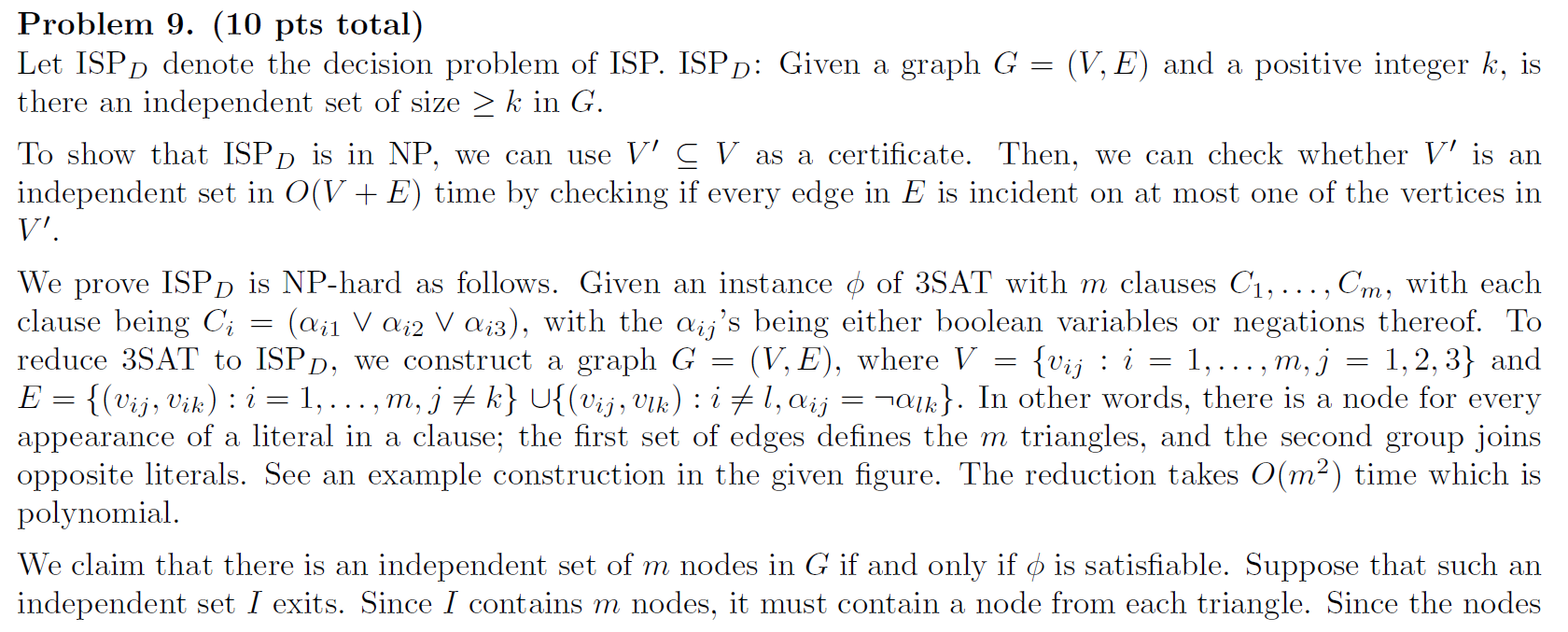
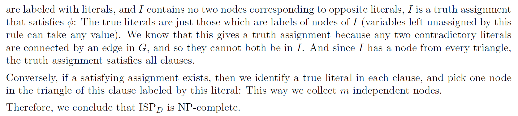
independent set
- a subset \(V'\subseteq V\) s.t. no edge between any nodes in \(V'\)
- independent-set problem
- problem: Is there an independent set of size \(\geq\) k?
- 3SAT to independent-set decision problem
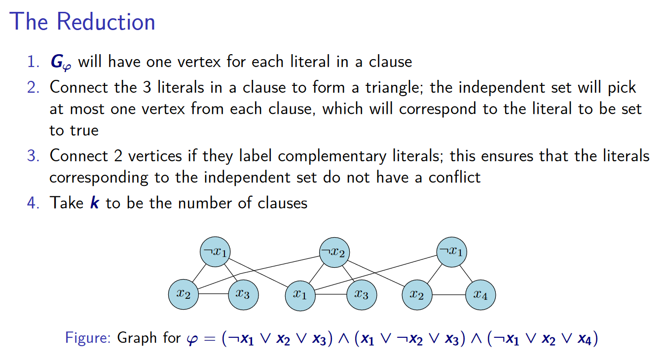
- https://courses.engr.illinois.edu/cs374/fa2020/lec_prerec/23/23_2_0_0.pdf
- 每個三角形選一個 node 作為 true,選到的 node 就是 independent set
- 不可能同時選 x & x' → 把 x & x' 連在一起 s.t. independent set 不會有 conflict 的 nodes
hitting set
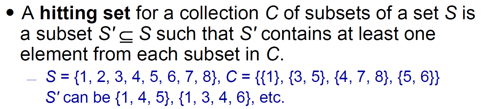
- for all \(c\in C\), \(c\) 的元素至少有一個在 \(S'\)
- hitting-set problem
- Does S contain a hitting set for C of size \(\leq\) k?
- reduction to vertex cover
- restrict each \(c\in C\) to have size of 2
- each \(c\) is an edge in clique
- \(S'\) 是 vertex cover 的 node 指到的每個 node
- restricted 版本是 NP-Complete → unrestricted 版本是 NP-Complete
approx TSP
- NP