Econometrics
resources
- Econometrics Midterm
- problems & my answer
- Econometrics Midterm Solution
- Econometrics Final
notation and stuff
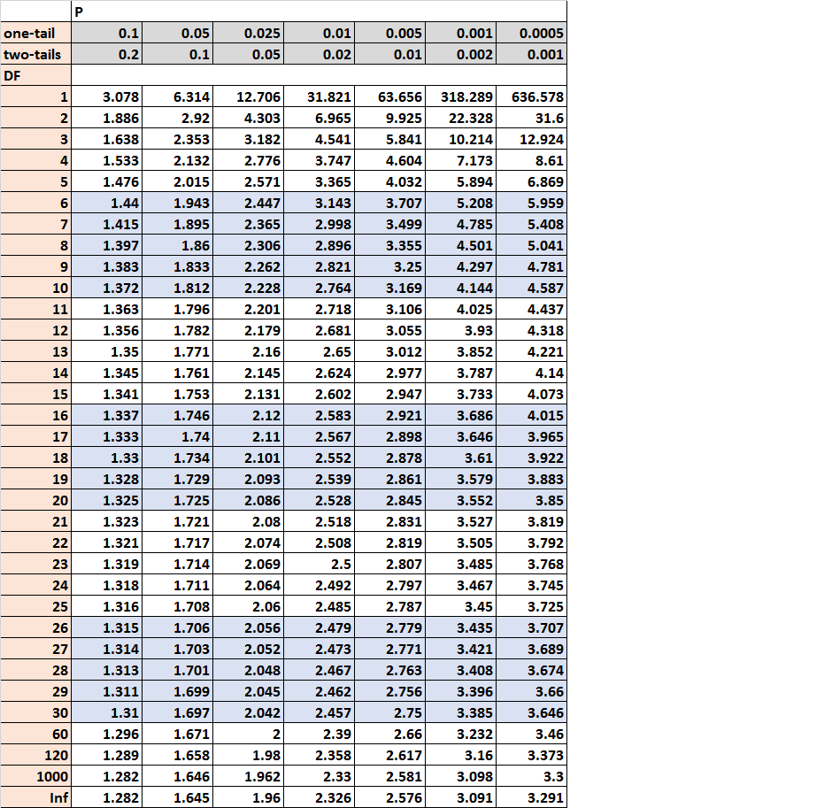
- CI
- 99%: 2.5758 = 2.576 = 2.58
- 95%: 1.9600 = 1.960 = 1.96
- 90%: 1.6449 = 1.645 = 1.65
- df: degree of freedom
- coefficient
- the slope of each regressor
- estimate
- the estimate value
- sum(each regressor x its coefficient)
review of probability
correlation & independence
- uncorrelated is weaker than independent
- E(X)(Y)=E(XY) \(\iff\) uncorrelated
- P(X)(Y)=P(XY) \(\iff\) independent \(\Longrightarrow\) uncorrelated
- https://www.themathcitadel.com/uncorrelated-and-independent-related-but-not-equivalent/
skewness
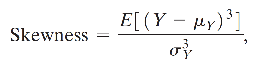
The skewness of a symmetric distribution is 0.
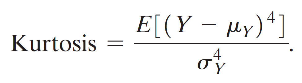
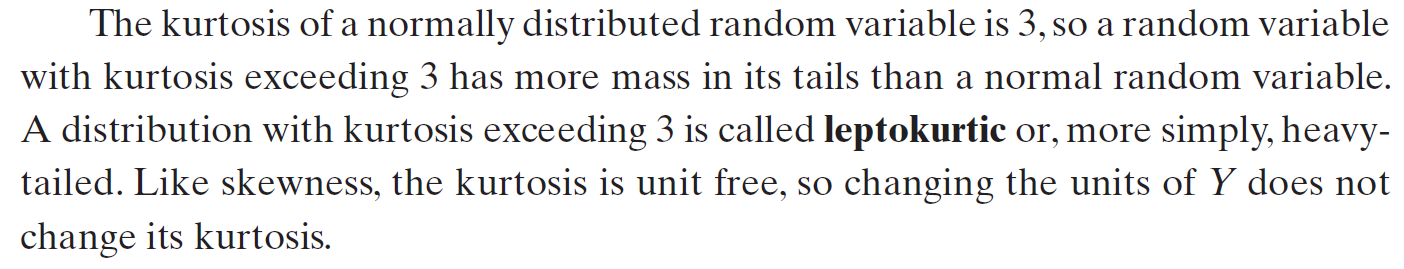
kurtosis
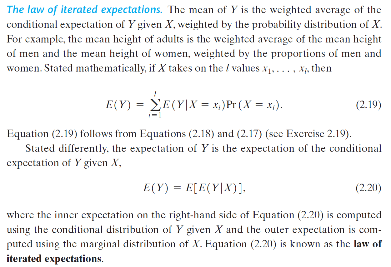
law of iterated expectations
Ch3 review of statistics
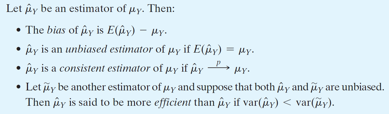
- unbiasedness
- bias = \(E(\hat{\mu_Y})-\mu_Y\)
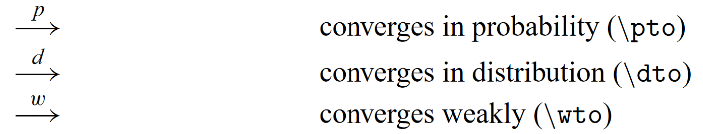
- consistency
- \(\hat{\mu_Y}\) → \(\mu_Y\) on large sample
- efficency
- lower variation → higher efficency
- standard error, SE
- std for sample
- \(\hat{p}\)
- p for sample
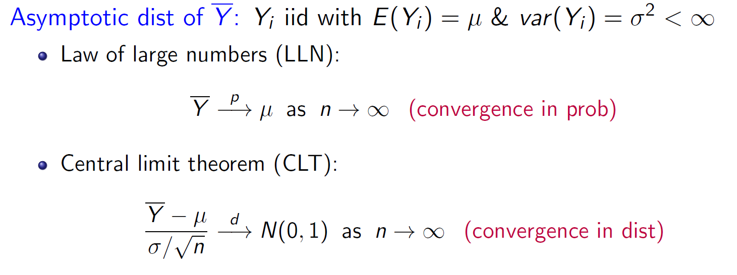
- central limit theoreom
- \(\dfrac{\bar{Y}-\mu}{\frac{\sigma}{\sqrt{n}}} →N(0,1)\) as \(n → \infty\)
null hypothesis & alternate hypothesis
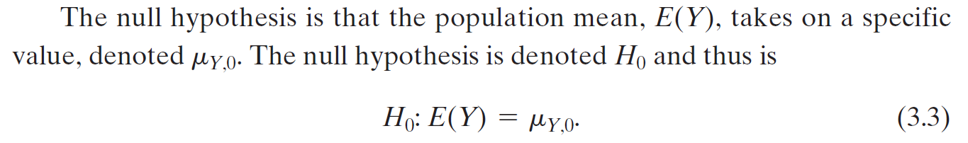
\(E(Y) = \mu_Y\) → null hypothesis
\(E(Y) \neq \mu_Y\) → (two-sided) alternate hypothesis
How to describe a testing result
There is (no) statistically significant evidence that ...... at the 1%/5%/10% level
p-value
- significance probability
- \(t^{act}=\frac{\hat{\mu_y}-\mu_y}{\sigma_y}\)
- 抽樣平均在理論平均的 t 個標準差外的機率 → null hypothesis 正確機率
i.e. \(2(1-\Phi(\frac{\hat{\mu_y}-\mu_y}{\sigma_y}))\) if N(0,1)
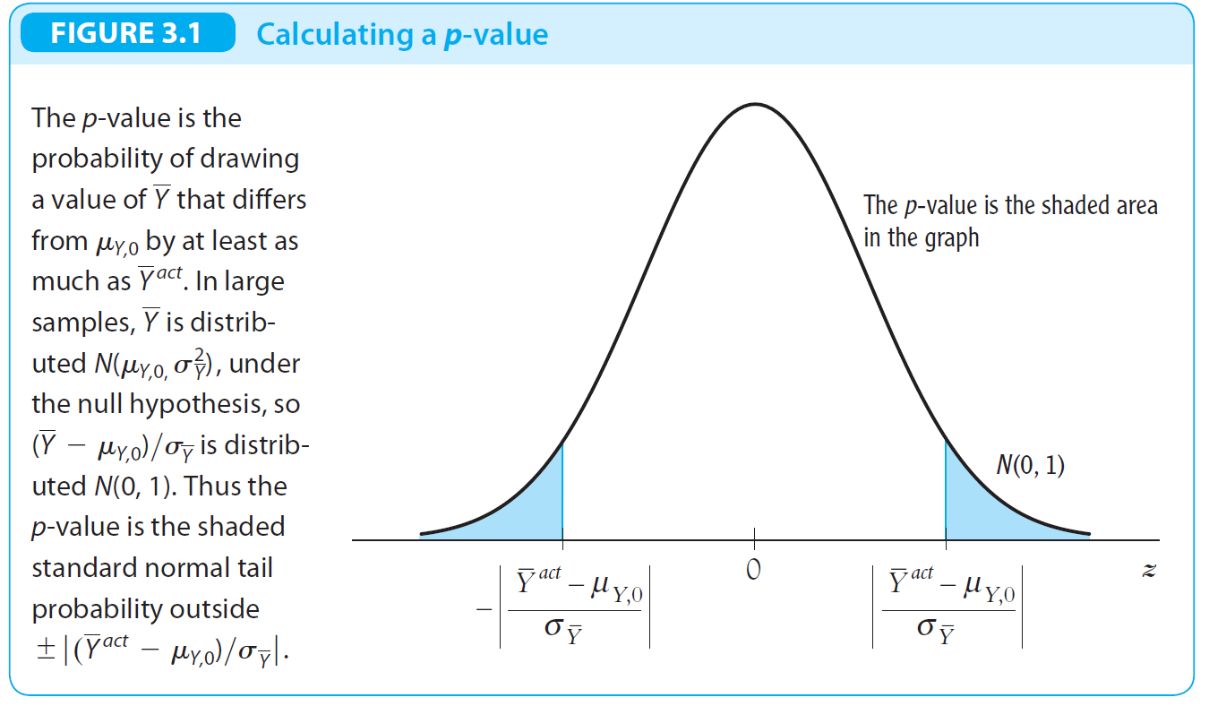
- 假設抽樣算出的平均,去根據 null hypothesis 的 mean 算出 p-value 很小,i.e. 抽樣平均離理論平均很遠,那麼 null hypothesis 就很有可能是錯誤的,i.e. 理論平均應該不是那樣; 反之,若 p-value 很大,則 null hypothesis i.e. 理論平均很有可能是正確的
-
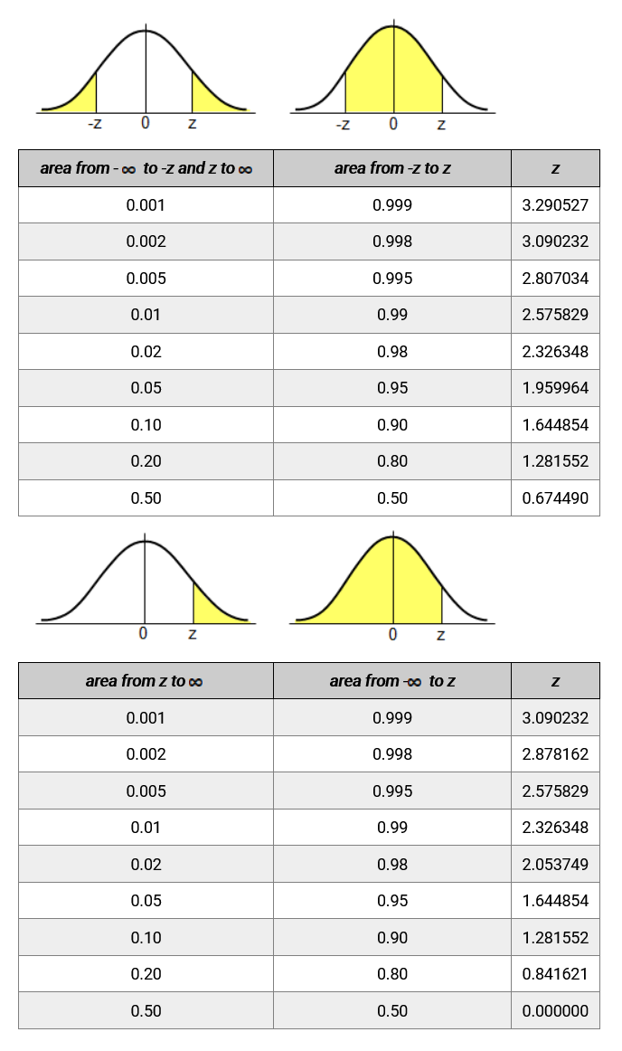
if p-value < 5% → reject the null hypothesis
- for two-sided, p-value < 0.05 i.e. \(|t^{act}|>1.96\) (\(\Phi(1.96)=0.975\))
- for one-sided, p-value < 0.05 i.e. \(|t^{act}|>1.64\) (\(\Phi(1.64)=0.95\))
- meaning you would incorrectly reject the null hypothesis once in 20 cases on average
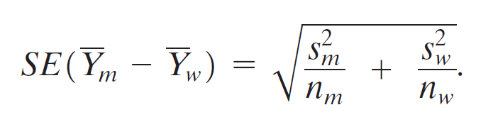
-
between two means
confidence interval
- \(\Phi(1.645)=95\%\)
- \(\Phi(1.96)=97.5\%\) → 95% confidence interval for two sided
- \(\Phi(2.576)=99.5\%\) → 99% confidence interval for two sided
(看 inf)
名詞
- size of a test
- the probability that a test incorrectly rejects the null hypothesis when the null hypothesis is true
- power of a test
- the probability that a test correctly rejects the null hypothesis when the alternative is true
Ch4 Linear Regression with One Regressor
- notations
- \(Y\): real sample value
- \(\hat{Y}\): predicted value
- \(\bar{Y}\): sample mean
- \(Y_i=\beta_0+\beta_1X_i+u_i\)
- \(u_i\): factor other than X (error term)
- if random assignment → \(E(u_i|X_i)=0\) → \(cov(u_i|X_i)=0\) i.e. \(u_i\) is not correlated to X
- correlation efficient
-
\[r_{XY}=\dfrac{s_{XY}}{s_Xs_Y}=\dfrac{\dfrac{1}{n-1}\displaystyle\sum_{i=1}^n(X_i-\bar{X})(Y_i-\bar{Y})}{\sqrt{\dfrac{1}{n-1}\displaystyle\sum_{i=1}^n(X_i-\bar{X})^2}\sqrt{\dfrac{1}{n-1}\displaystyle\sum_{i=1}^n(Y_i-\bar{Y})^2}}\]
-
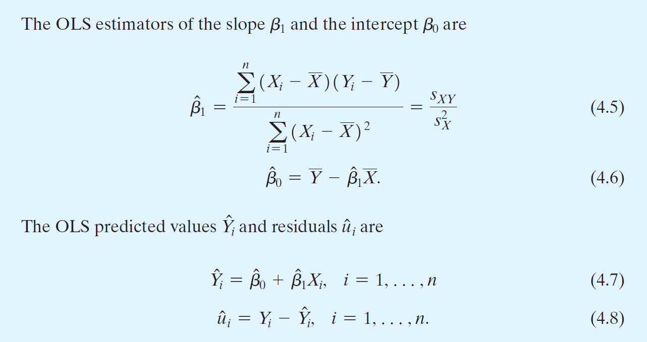
OLS
- \(\hat{\beta_0}\)、\(\hat{\beta_1}\): \(\beta_0\)、\(\beta_1\) minimalizing \(\displaystyle\sum_{i=1}^n(Y_i-\beta_0-\beta_1X_i)^2\)
- \(\hat{Y}=\hat{\beta_0}+\hat{\beta_1}\bar{X}\)
- \(Y_i=\hat{Y_i}+\hat{u_i}=\hat{\beta_0}+\hat{\beta_1}\bar{X}+\hat{u_i}\)
- formulas
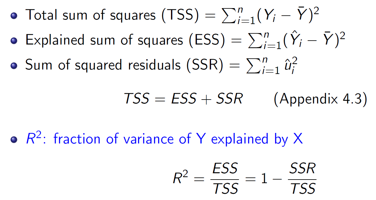
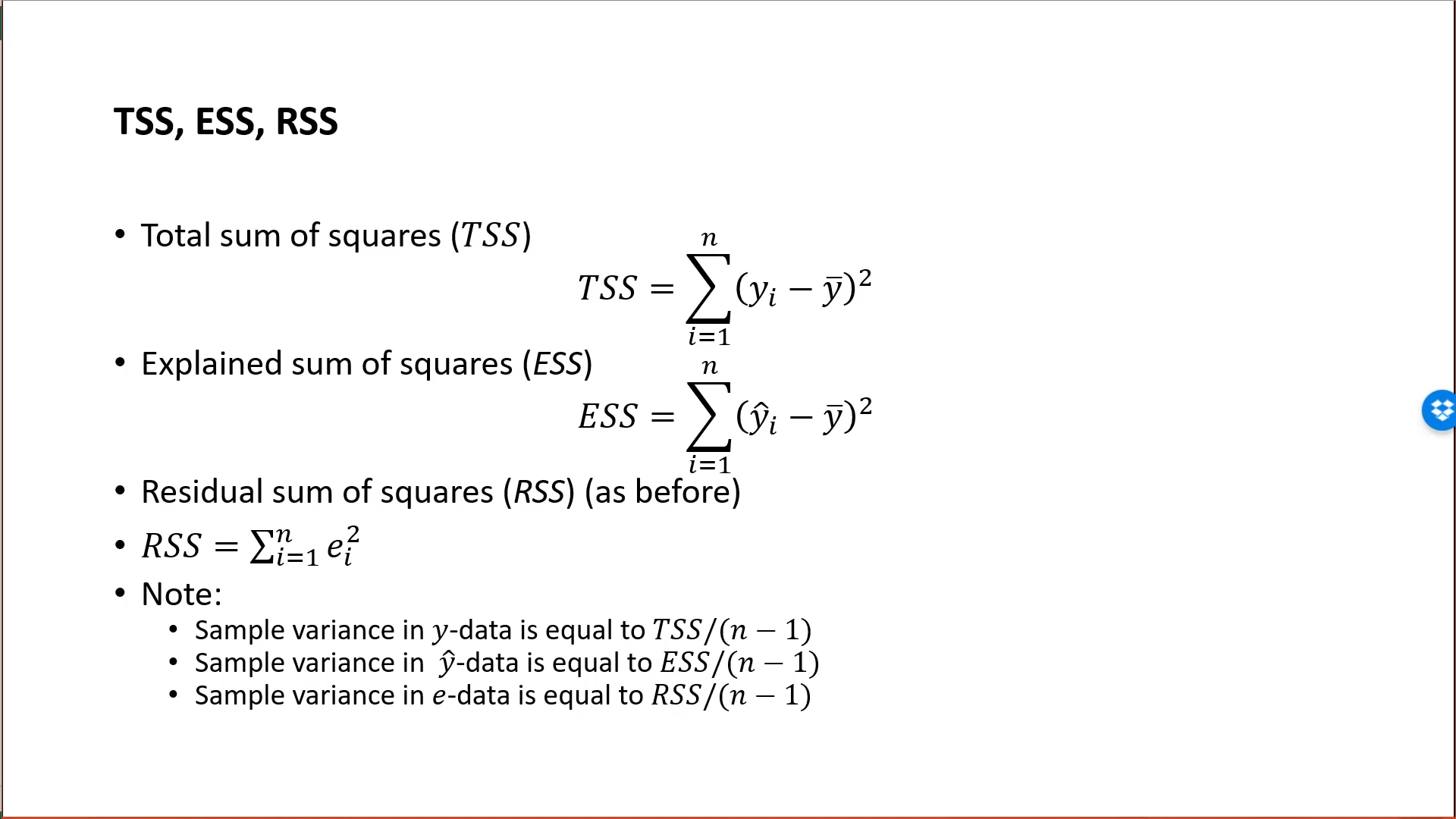
- total sum of squares \(TSS=\displaystyle\sum_{i=1}^n(Y_i-\bar{Y})^2\)
- explained sum of squares \(ESS=\displaystyle\sum_{i=1}^n(\hat{Y_i}-\bar{Y})^2\)
- sum of squared residuals \(SSR=\displaystyle\sum_{i=1}^n\hat{u_i}^2\)
- sample variance = \(\frac{TSS}{n-1}={s_Y}^2\)
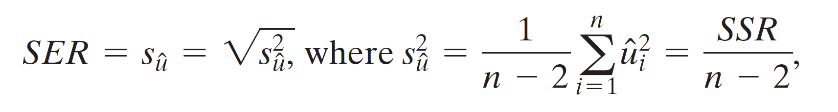
- \(SER=s_{\hat{u}}=\sqrt{\frac{SSR}{n-2}}\)
- SER: standard error of regression
- \(s_{\hat{u}}\): standard error of \(u_i\)
- \(TSS=ESS+SSR\)
- \(R^2=\frac{ESS}{TSS}=\frac{TSS-SSR}{TSS}=1-\frac{SSR}{TSS}\)
- degree of freedom
- variance degree of freedom is n-1 as the sample mean is decided → only n-1 sample values is free
- SER, standard error of the regression
- standard error of \(u_i\)
\(R^2\)
- correlation efficient \(^2\)
- fraction of Var(Y) explained by X
- both X and \(u_i\) contributes to Var(Y)
\(\Delta\) adjusted R-squared
Let us first understand what is R-squared: R-squared or R2 explains the degree to which your input variables explain the variation of your output / predicted variable. So, if R-square is 0.8, it means 80% of the variation in the output variable is explained by the input variables. So, in simple terms, higher the R squared, the more variation is explained by your input variables and hence better is your model.
However, the problem with R-squared is that it will either stay the same or increase with addition of more variables, even if they do not have any relationship with the output variables. This is where “Adjusted R square” comes to help. Adjusted R-square penalizes you for adding variables which do not improve your existing model.
Hence, if you are building Linear regression on multiple variable, it is always suggested that you use Adjusted R-squared to judge goodness of model. In case you only have one input variable, R-square and Adjusted R squared would be exactly same. Typically, the more non-significant variables you add into the model, the gap in R-squared and Adjusted R-squared increases. https://discuss.analyticsvidhya.com/t/difference-between-r-square-and-adjusted-r-square/264/3
不懂, 為何加 data 點 R-squared 就一定會不變 or 上升
- least square assumptions
Ch5 Multiple Regressor
- more regressor → \(R^2\) \(\uparrow\) as SER \(\downarrow\)
- adjusted \(R^2\)
- \(\bar{R}^2=1-\dfrac{n-1}{n-k-1}\dfrac{SSR}{TSS}\)

- k: regressor 數量 (對 k=1 的時候 \(\bar{R}^2\) 不一樣)
- adjusted \(R^2\)
- omitted variable bias
- 影響的眾多因素之間可能非 independent → 用較少 regressor 的話會 overestimate 那個 regressor 的影響
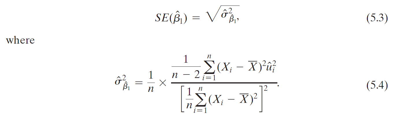
- standard error of \(\hat{\beta}\)
- binary variable
- alias
- indicator variable
- dummy variable
- alias
- contonious variable
- 與 binary variable 相對
homoskedastic & heterosketasdic
- homoskedastic
- if \(var(u_i|X_i)\) doesn't depend on \(X_i\)
- heterosketasdic
- if \(var(u_i|X_i)\) depends on \(X_i\)
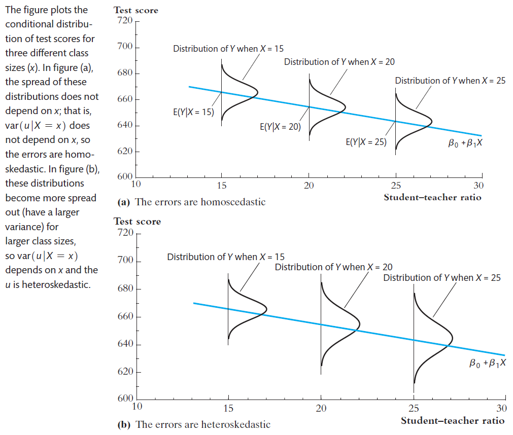
- heterosketasdic 的 distribution 因 x 而異
Ch6 Linear Regression with Multiple Regressors
treat intercept as a regressor

omitted variable bias
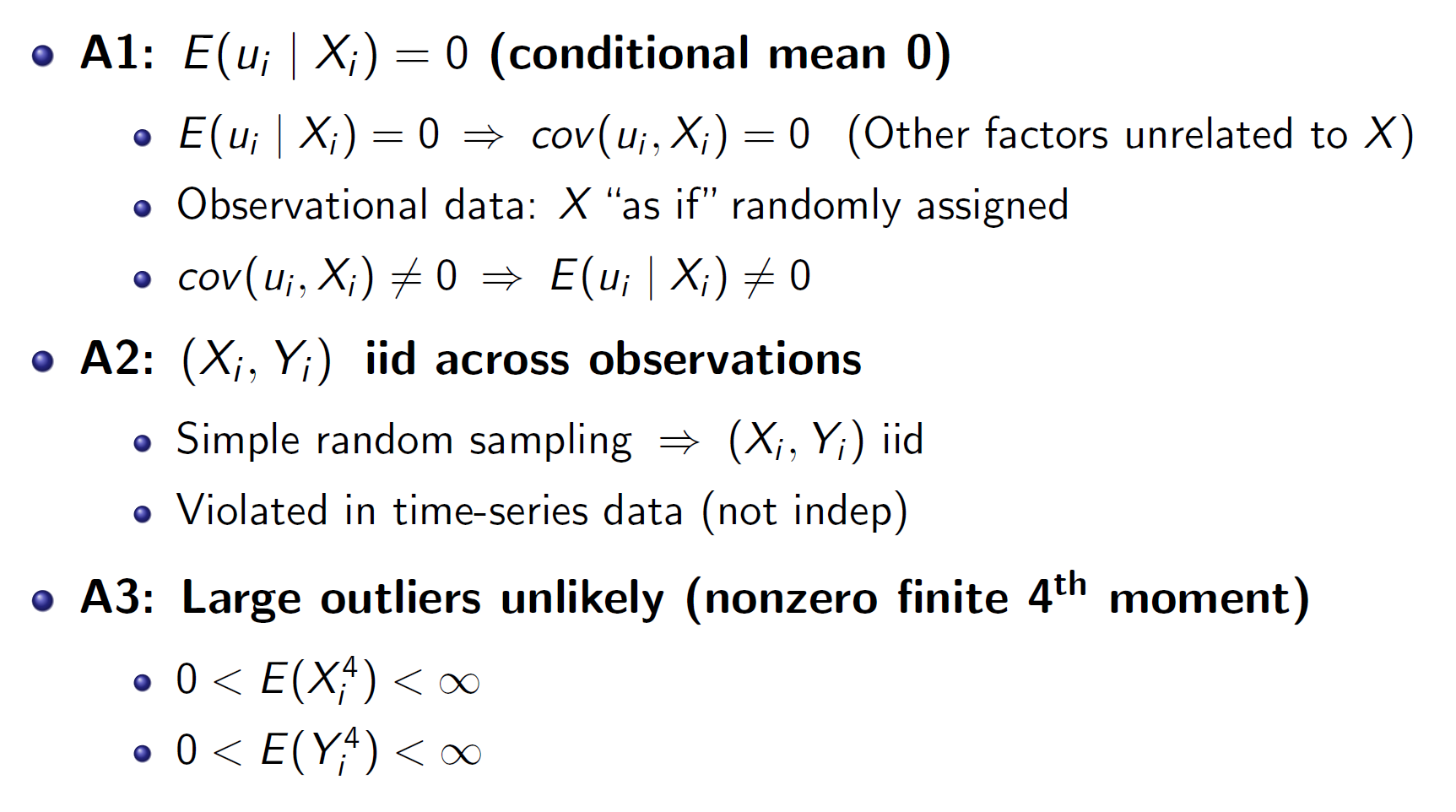
least square assumptions
- Assumption 1: The Conditional Distribution of ui Given X1i, X2i, . . . , Xki Has a Mean of 0
- Assumption 2: (X1i, X2i, . . . , Xki, Yi), i = 1, . . . , n, Are i.i.d.
- Assumption 3: Large Outliers Are Unlikely
- Assumption 4: No Perfect Multicollinearity
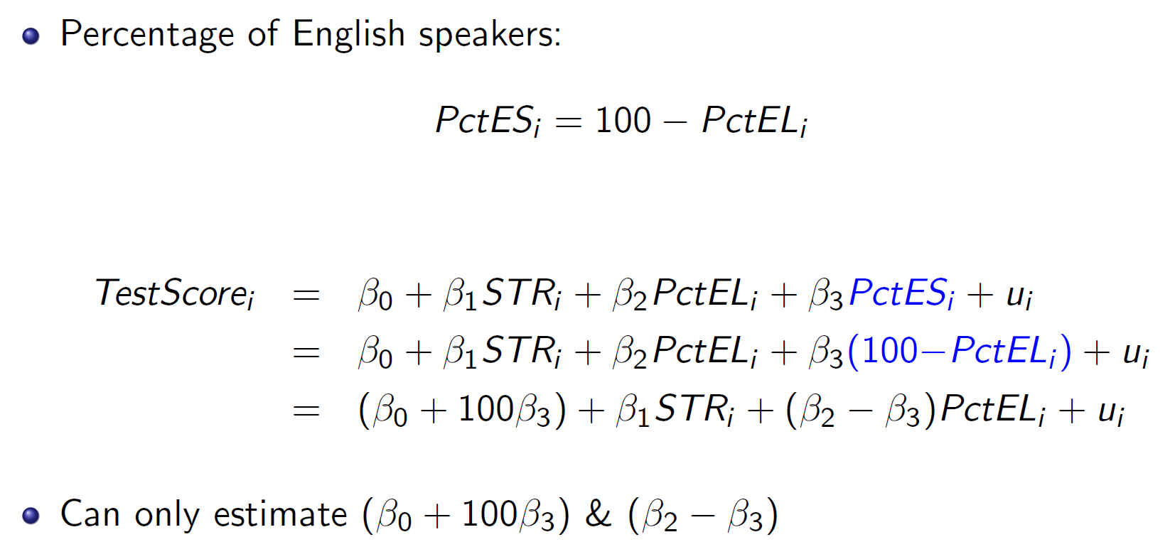
- if one of the regressors is a perfect linear function of the other regressors → perfect multicollinearity
- multiple regression: 其他 regressor 不動,只動這一個 → 不合理 when one variable is a linear function to another
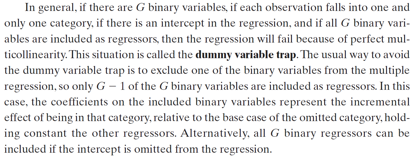
- dummy variable trap
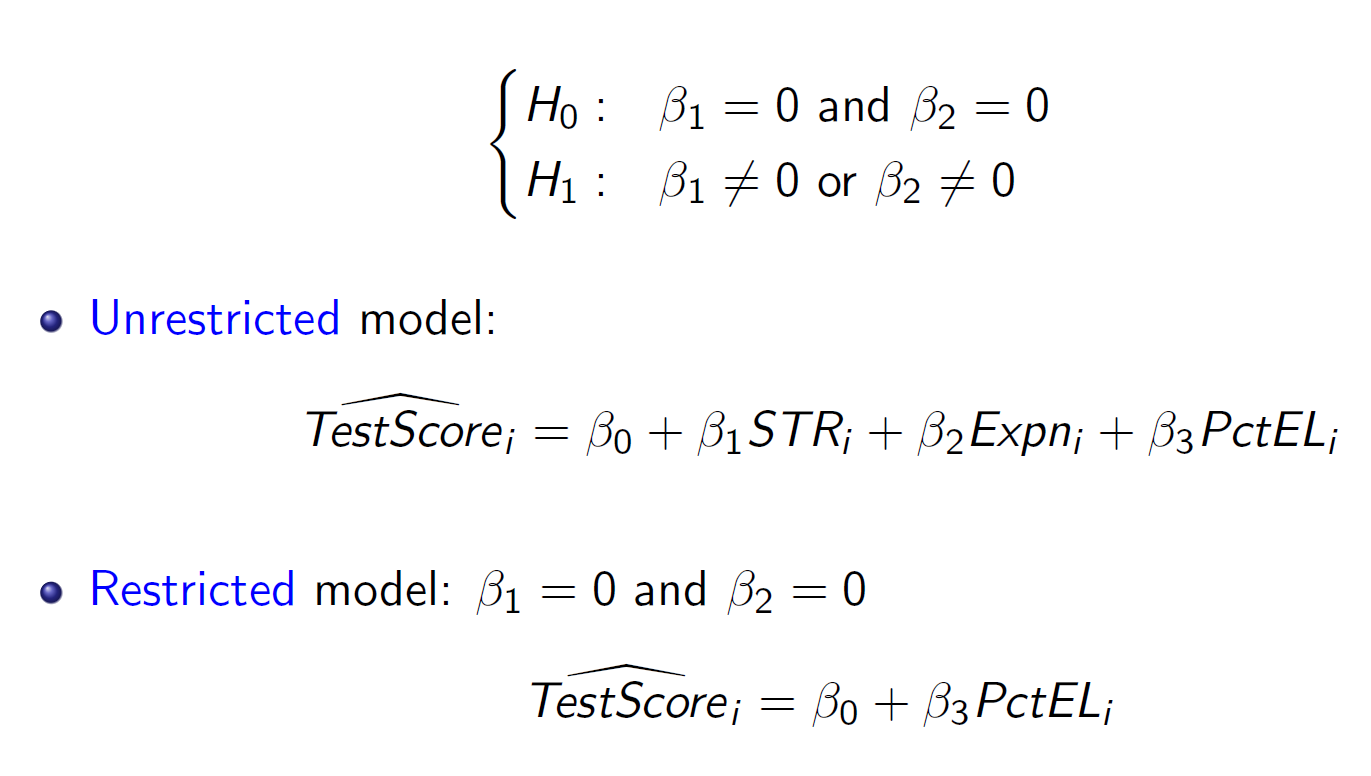
Ch7 Hypothesis Tests & Confidence Intervals in Multiple Regression
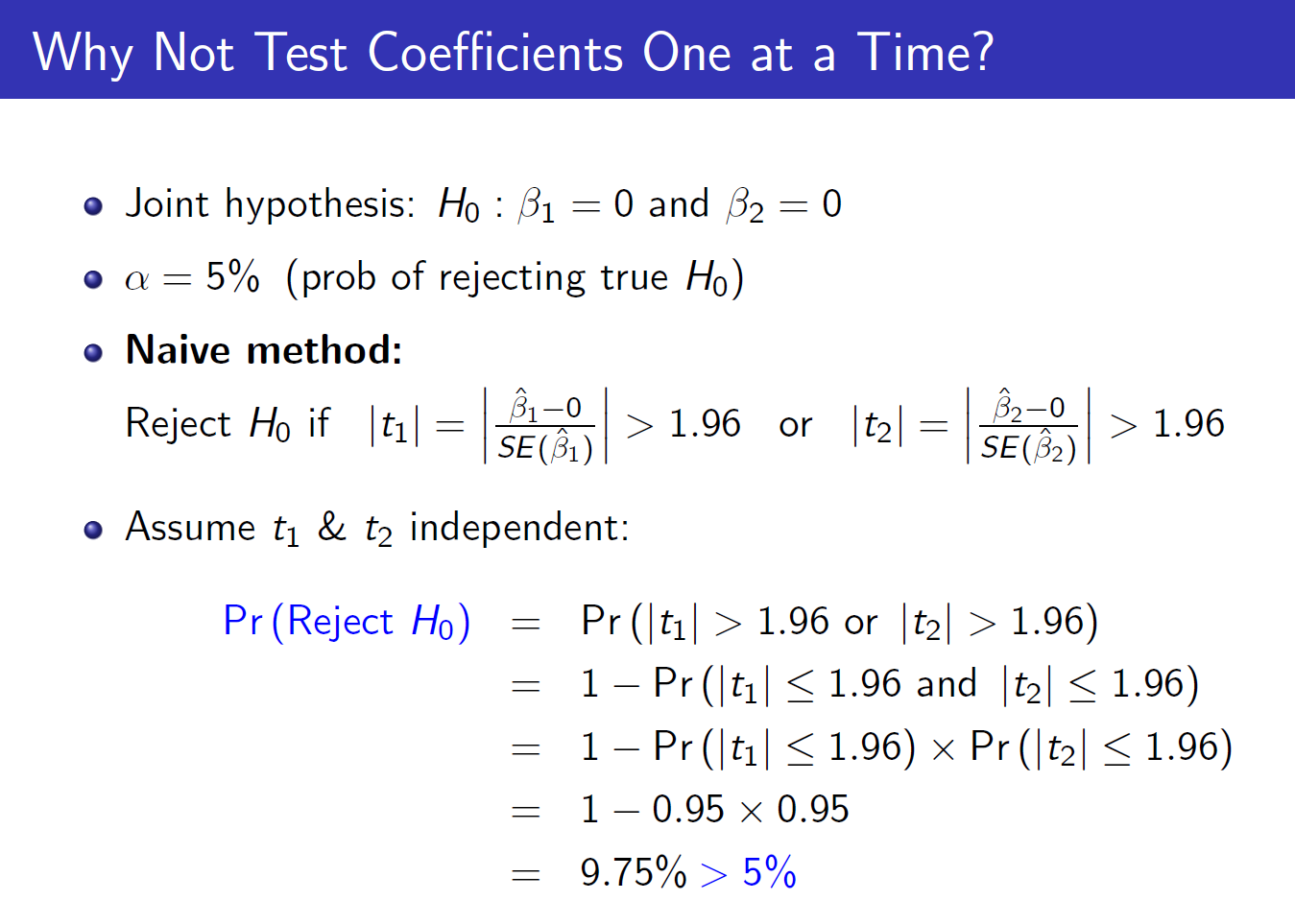
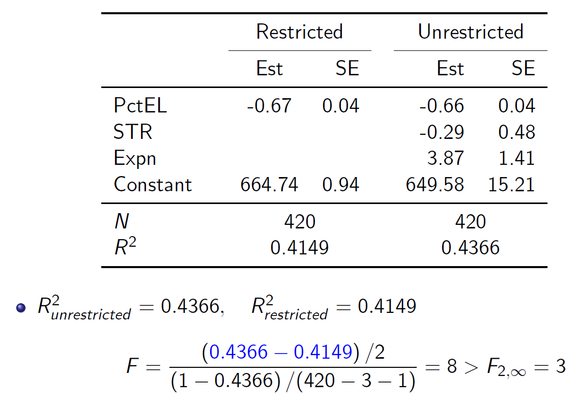
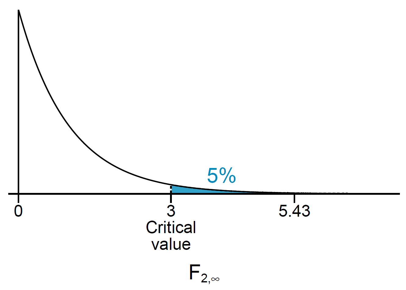
- F test
- for multiple regressors
- table
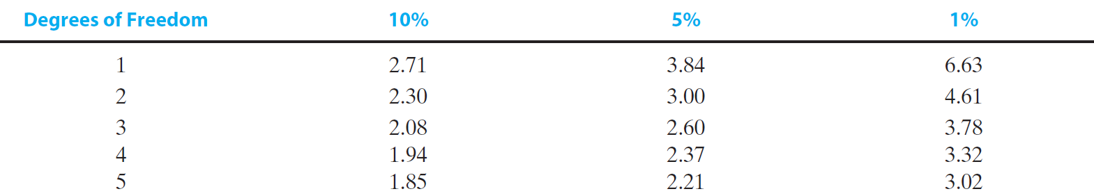
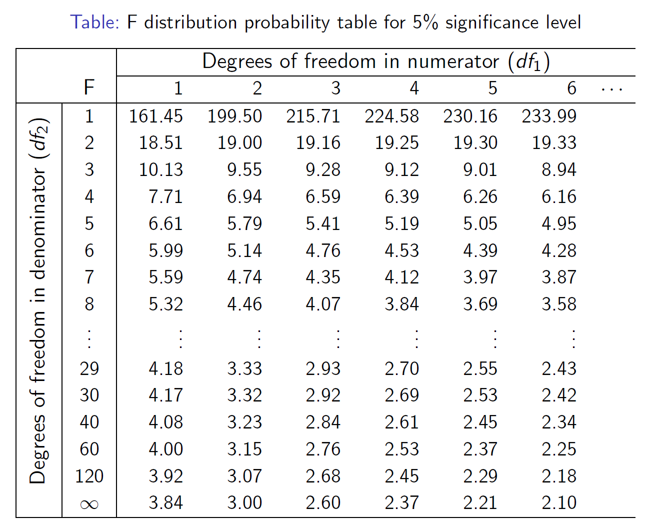
- e.g. \(f_{2,\infty}\)=3
- for 2 regressors, \(F^{act}\) for 5% is 3
- F-stat restricted & unrestricted
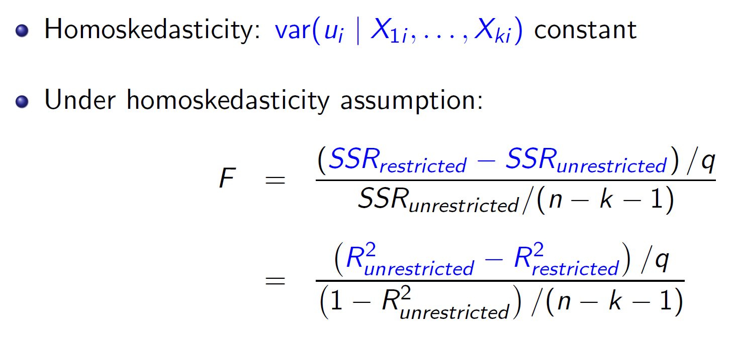
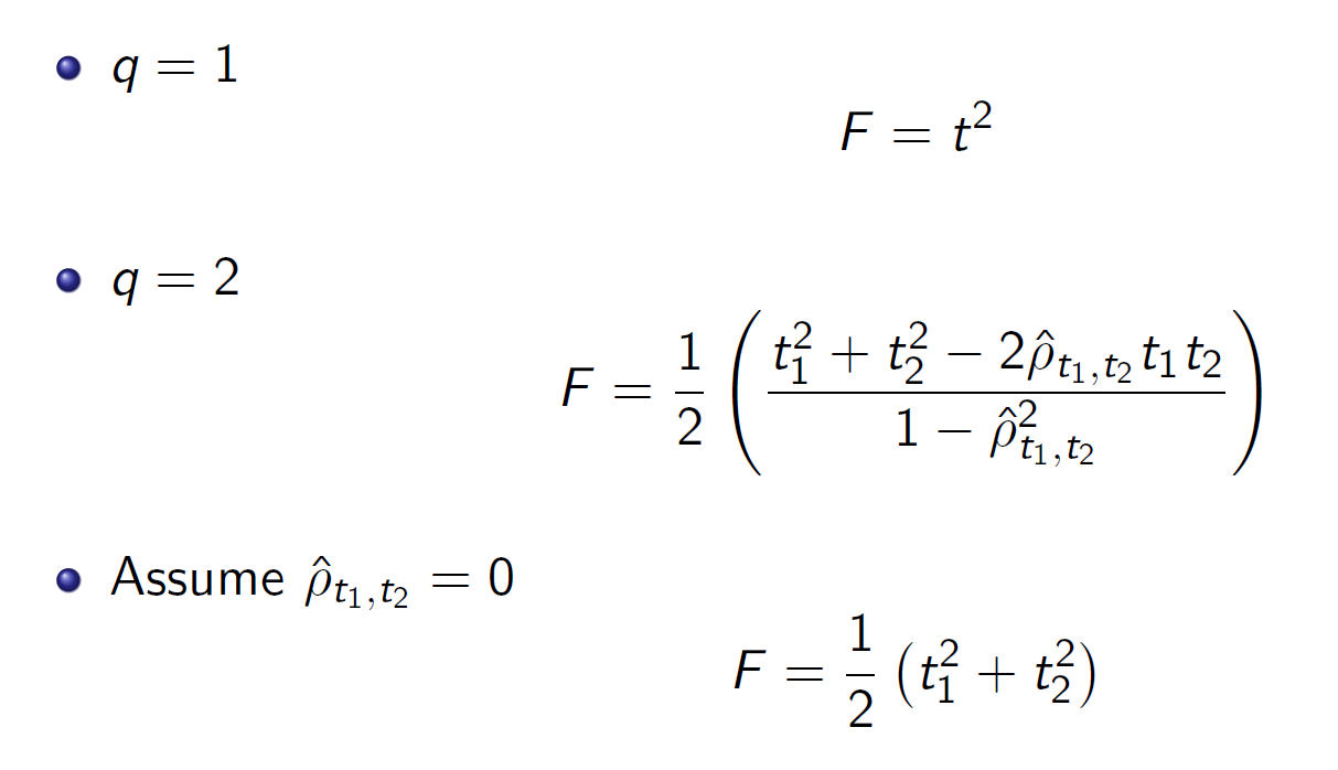
- q = num of restrictions under the null
- k = num of regressor of the unrestricted one
- Homoskedasticity
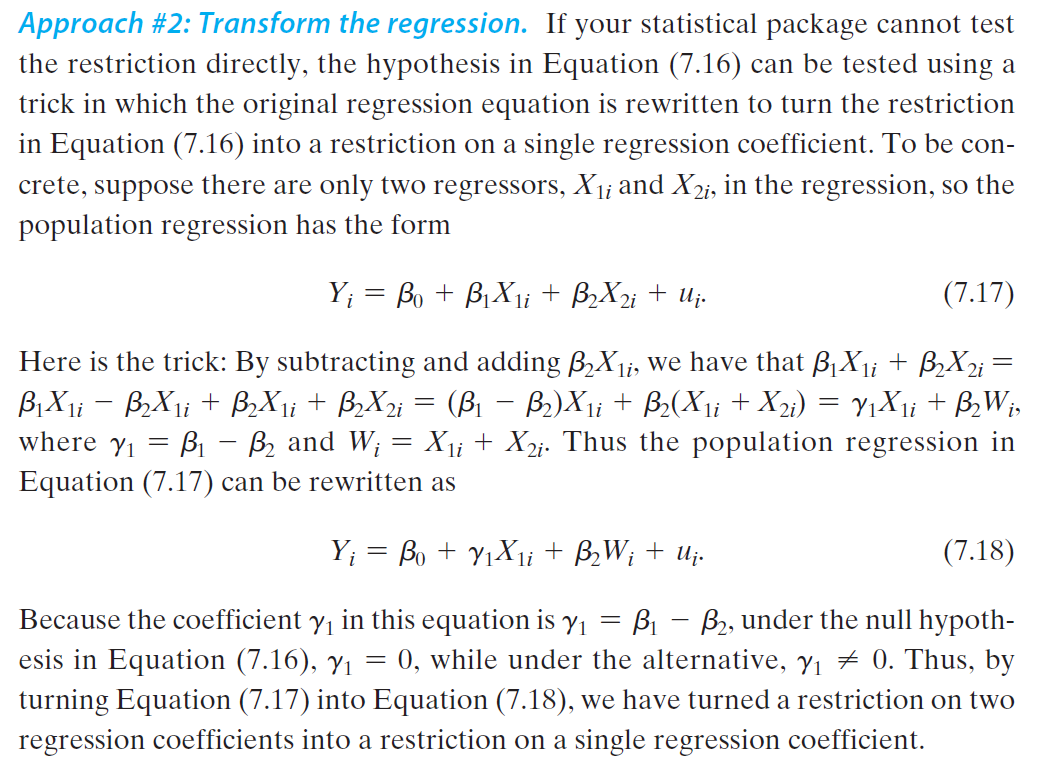
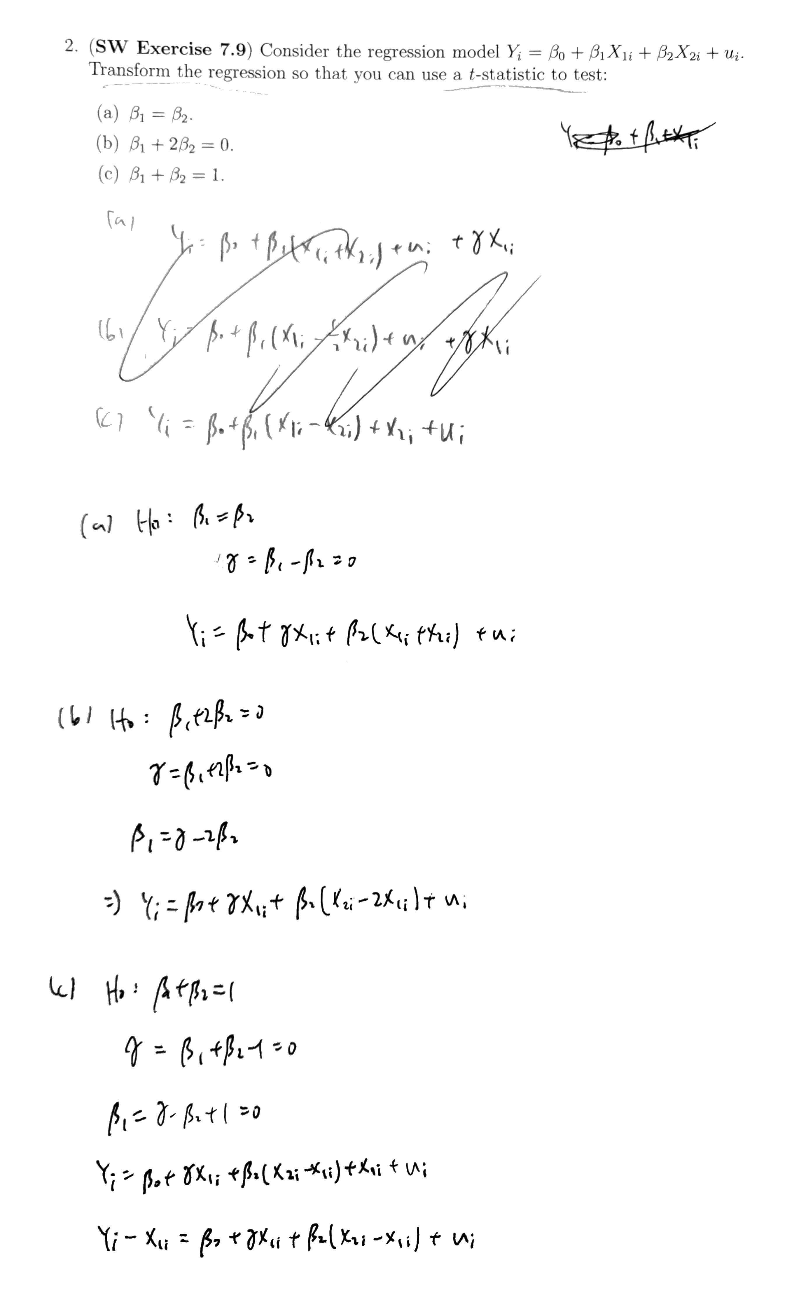
- turn multiple into singular
Ch8 nonlinear
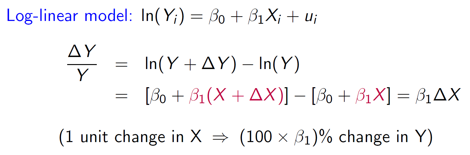
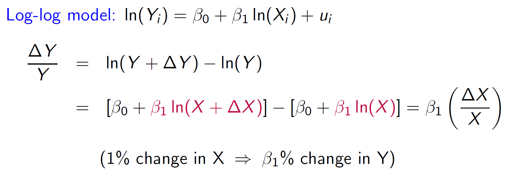
log
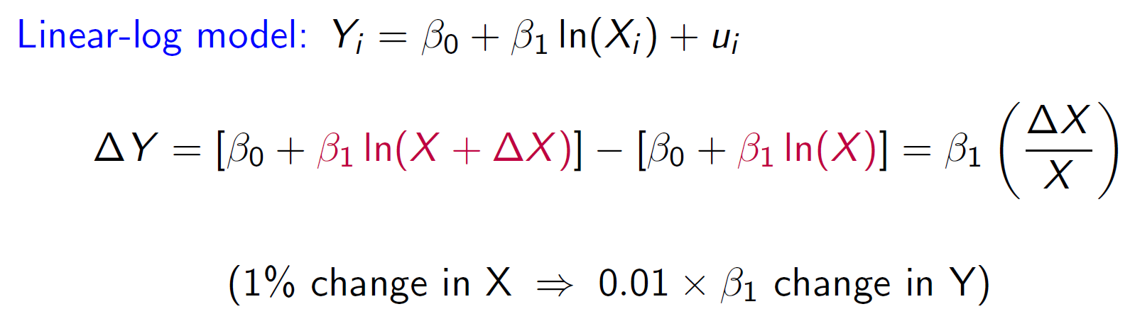
- bc \(\frac{ln(X+\Delta X)-ln(X)}{(X+\Delta X)-X}=\frac{dln(X)}{dX}=\frac{1}{X}\) → \(ln(X+\Delta X)-ln(X)=\frac{\Delta X}{X}\)
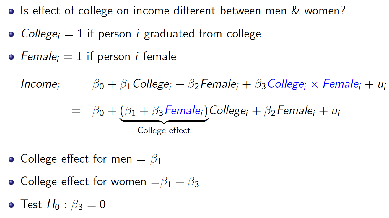
interaction variable
Ch9
simultaneous causality bias
- x 影響 y,y 也影響 x
- e.g.
- 有錢 → 吃得好用得好 → 正 → 機會比較多,也較可能嫁有錢人 → 有錢
- 景氣差 → 資產價格下跌 → 擔保品價值下降 → 外部融資溢酬增加 → 消費投資支出下降 → 景氣差
- 資源多 → 學生程度好 but 同時 學生程度差 → 政府給資源
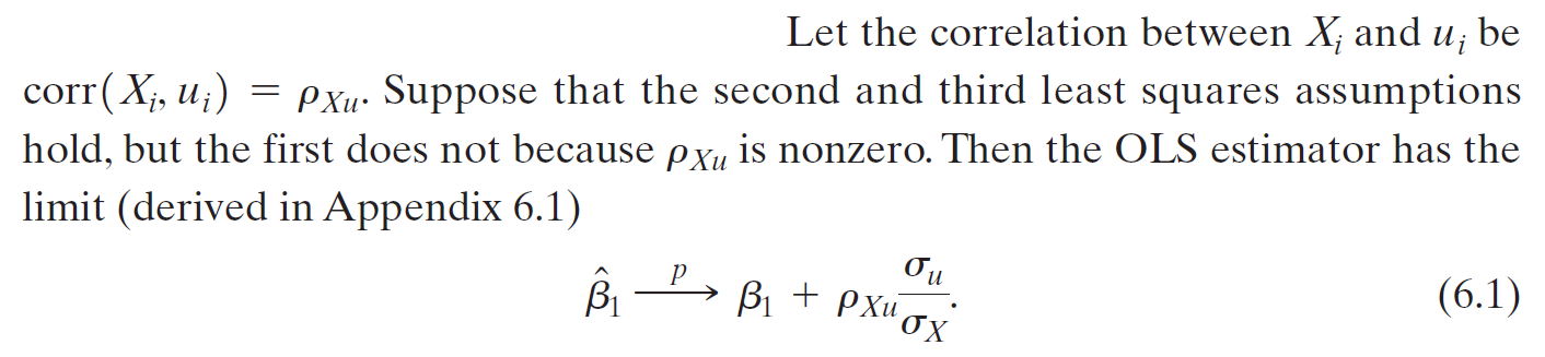
- 造成 corr(regressor, error term) != 0
- error term 影響 y, y 影響 x → error term 影響 x
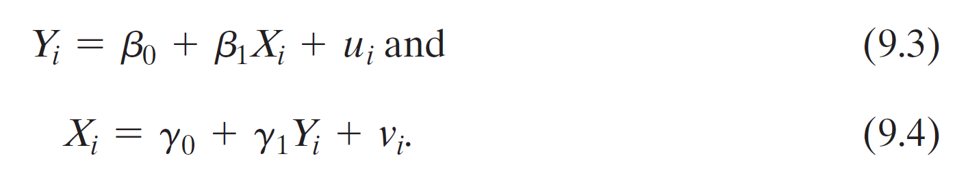
- (9.3) X cause Y
- (9.4) Y cause X
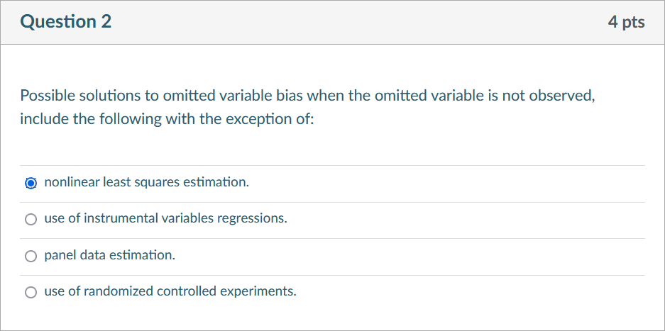
- solution
- use instrument (Ch12)
- design and implement a randomized controlled experiment in which the reverse causality channel is nullified (Ch13)
Ch10 panel data
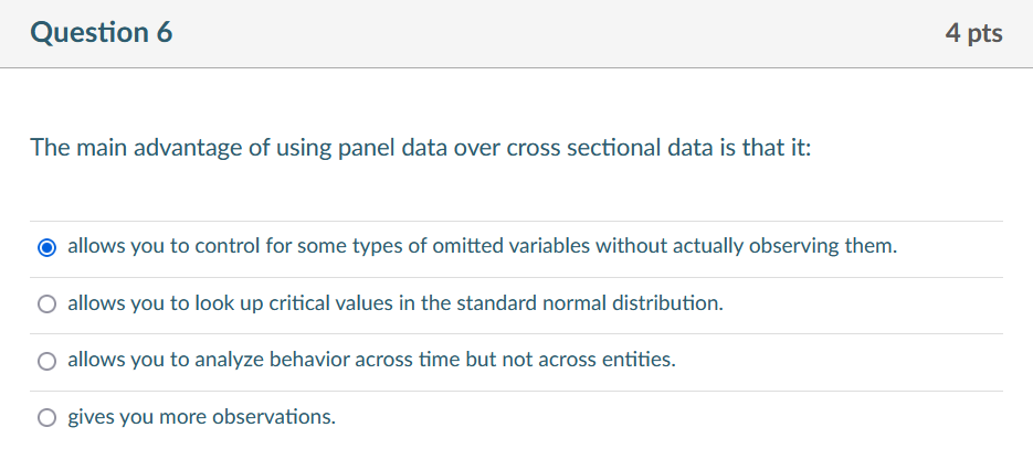
- panel data
- each observational unit, or entity, is observed at two or more time periods
- cross-sectional data
- one time different subject
- time series data
- one subject different time
- Standard errors should be clustered into groups within which the values of the dependent variable are likely to be correlated with one another.
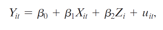
- fixed effects regression model
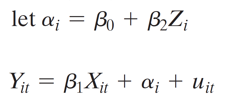

- omit \(D_1\) to avoid perfect multicollinearity
- \(\alpha_1\), \(\alpha_2\), ..., \(\alpha_n\):entity fixed effects
- comes from omitted variables, vary across entities (i) but not time (t)
- each treated as unknown intercepts to be estimated, one for each state
- \(Dx_i=\delta(x)\)
- \(\alpha_1=\beta_0\)
- \(\alpha_i=\beta_0+\gamma_i\) for i >= 2
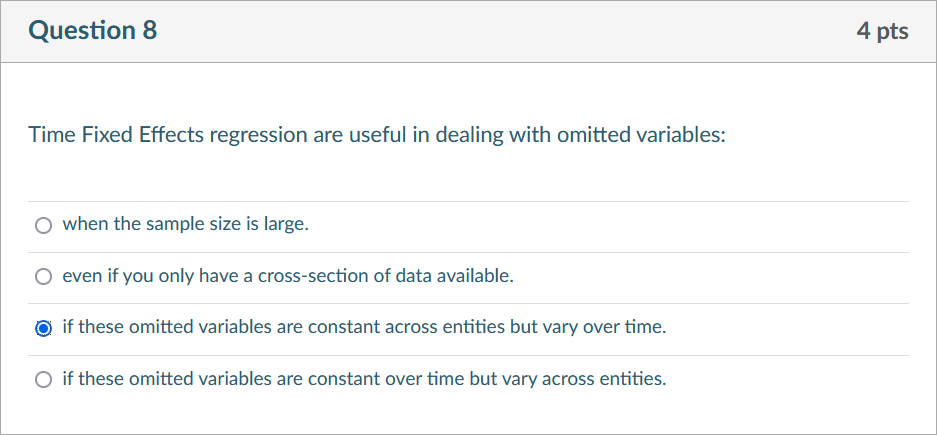
- time fixed effects regression model
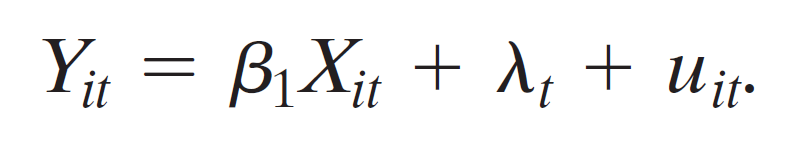
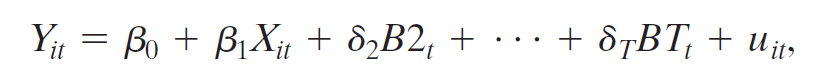
- omit \(B1_t\) to avoid perfect multicollinearity
- \(\lambda_1, ... \lambda_T\):time fixed effects
- comes from omitted variables, vary over time (t) but not entities (i)
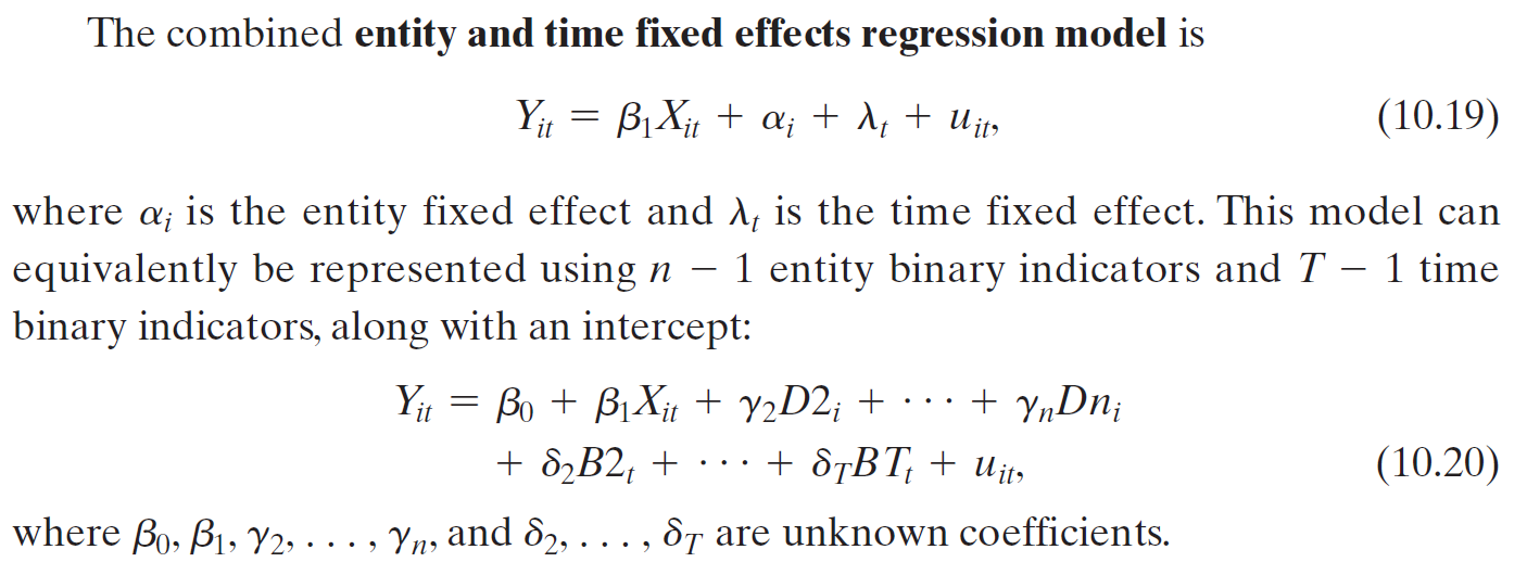
- entity and time effects regression model
Ch11 binary
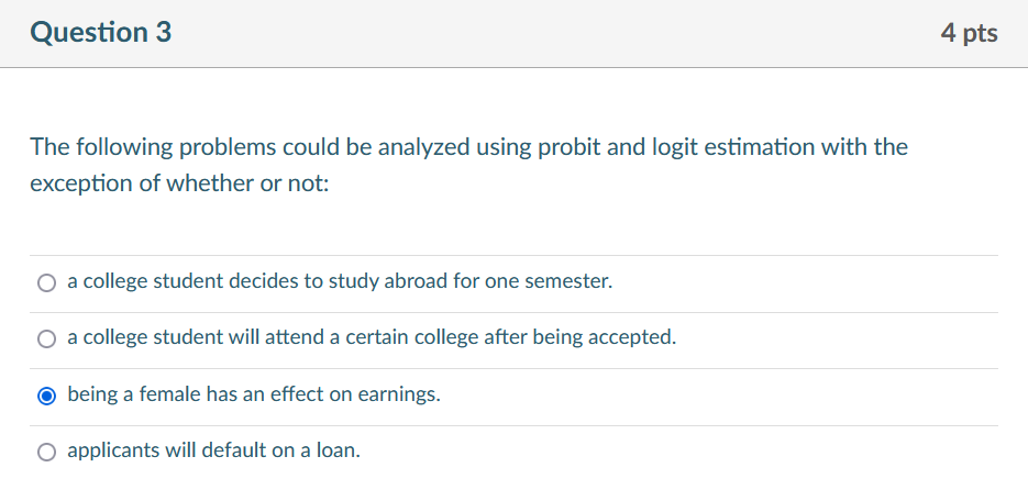
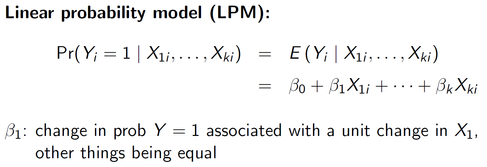
LPM linear
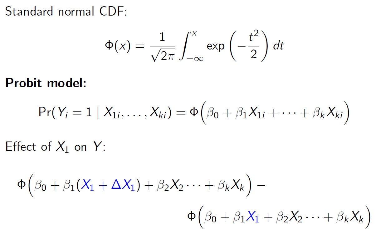
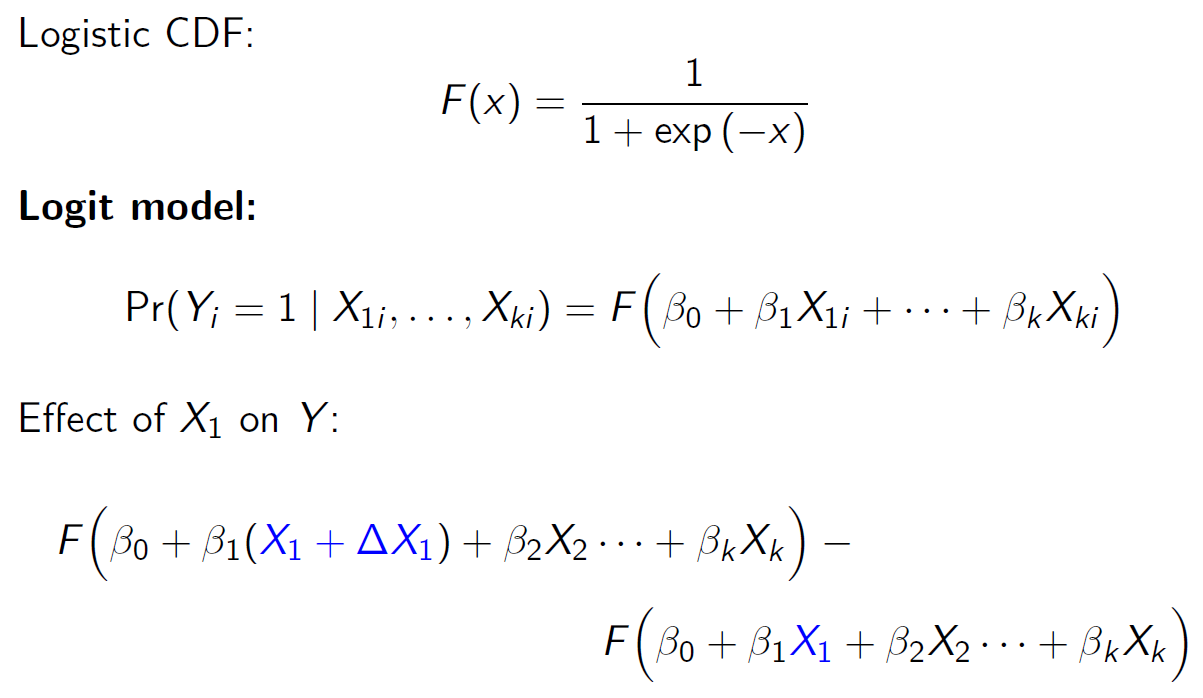
probit
logit
MLE maximum likelihood estimator
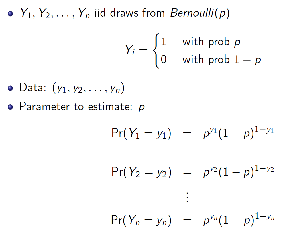
y1=1 → 1-y1=0
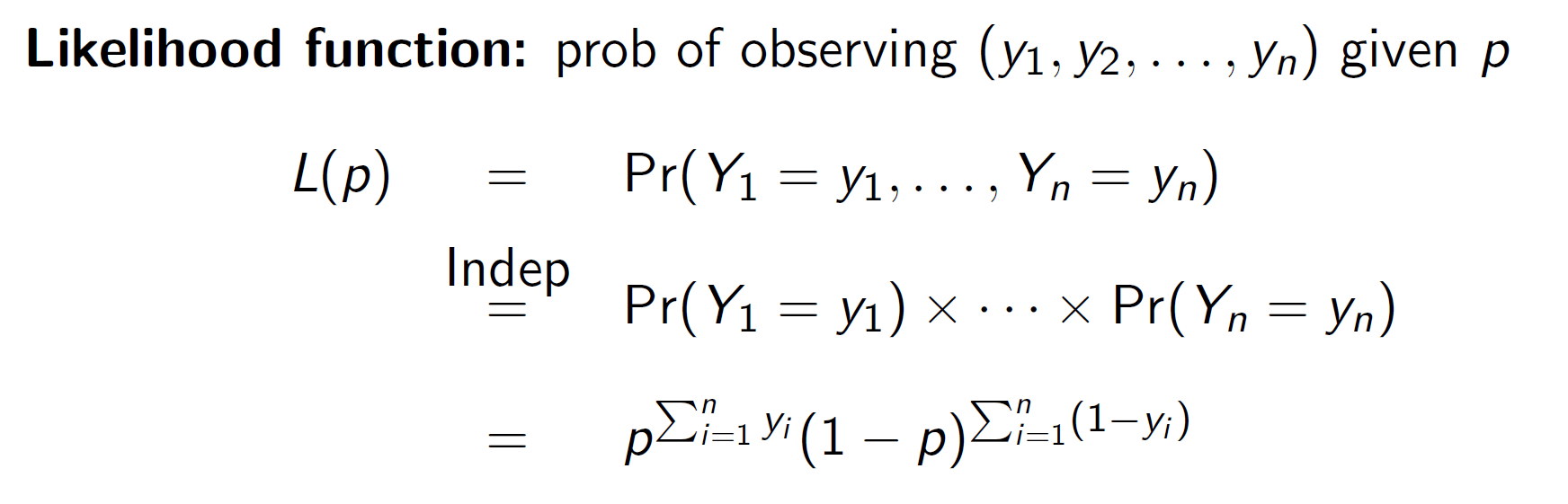
likelihood function
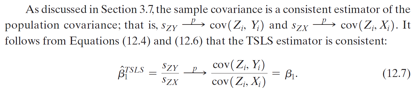
C12 Instrumental
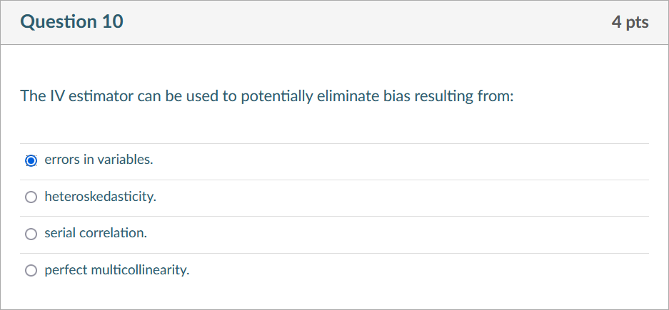
- exogenous: \(cov(X_i,u_i)=0\)
- endogenous: \(cov(X_i,u_i)\neq0\)
- X is correlated to u → find an instrument Z that is
- correlated to X (relevance)
- uncorrelated to u (exogeneity)
- Z 跟 Y 不直接相關,只是透過 X 影響 Y
- there are factors that will affect both X & u
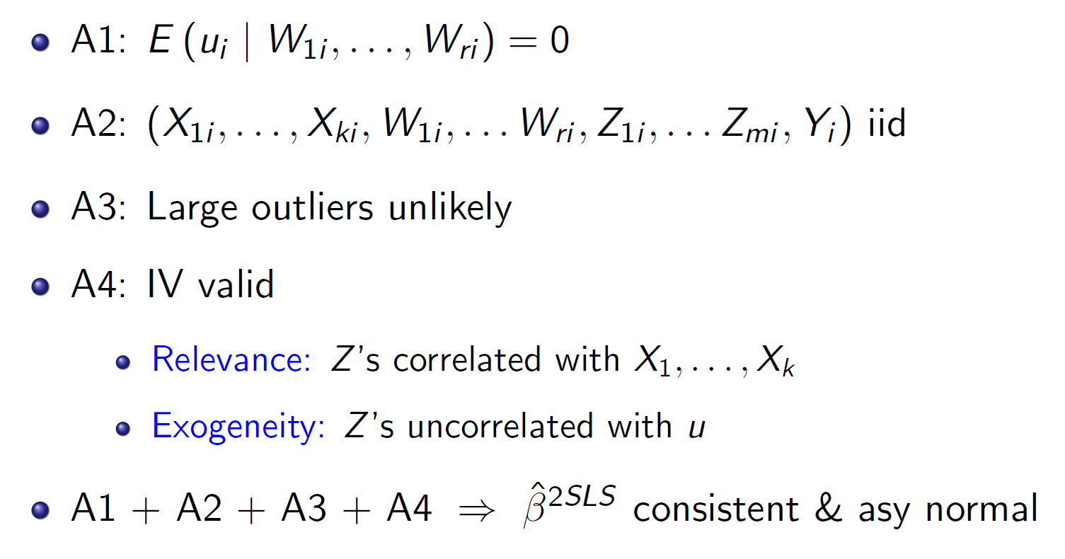
IV regression assumptions
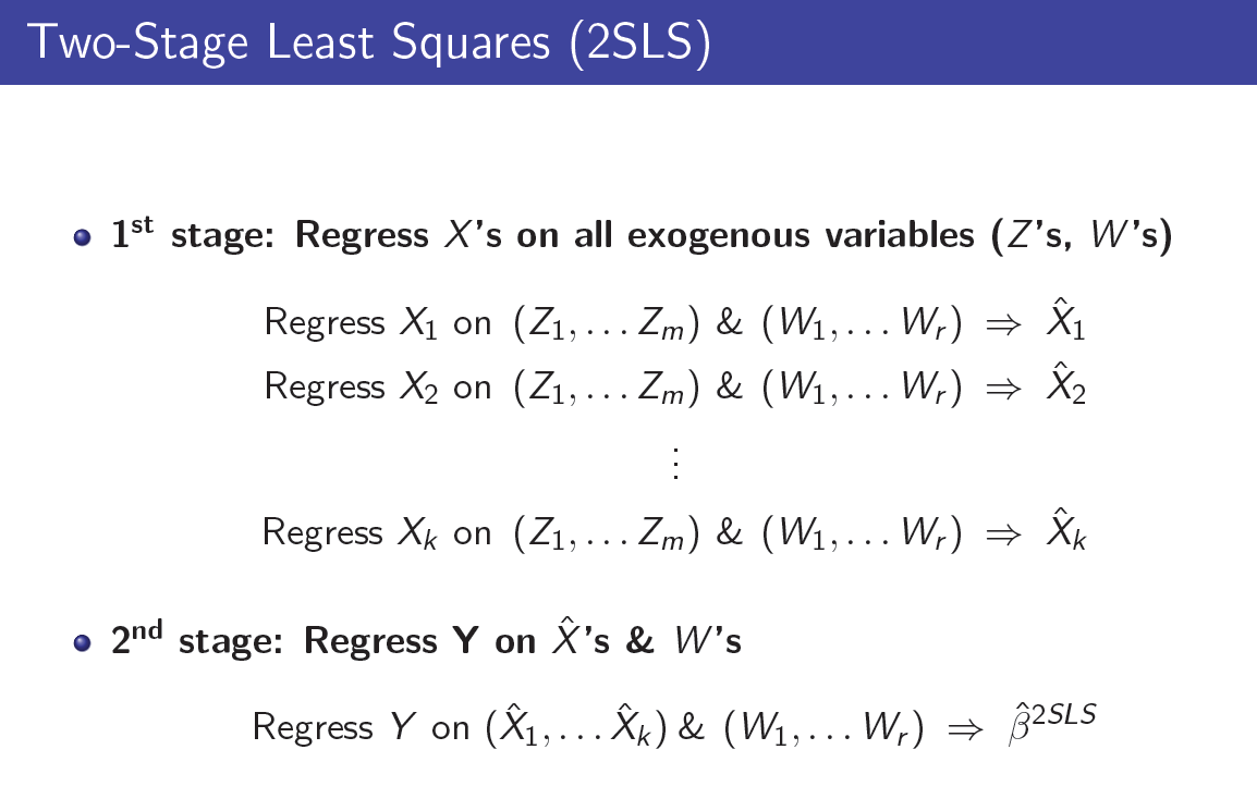
2SLS
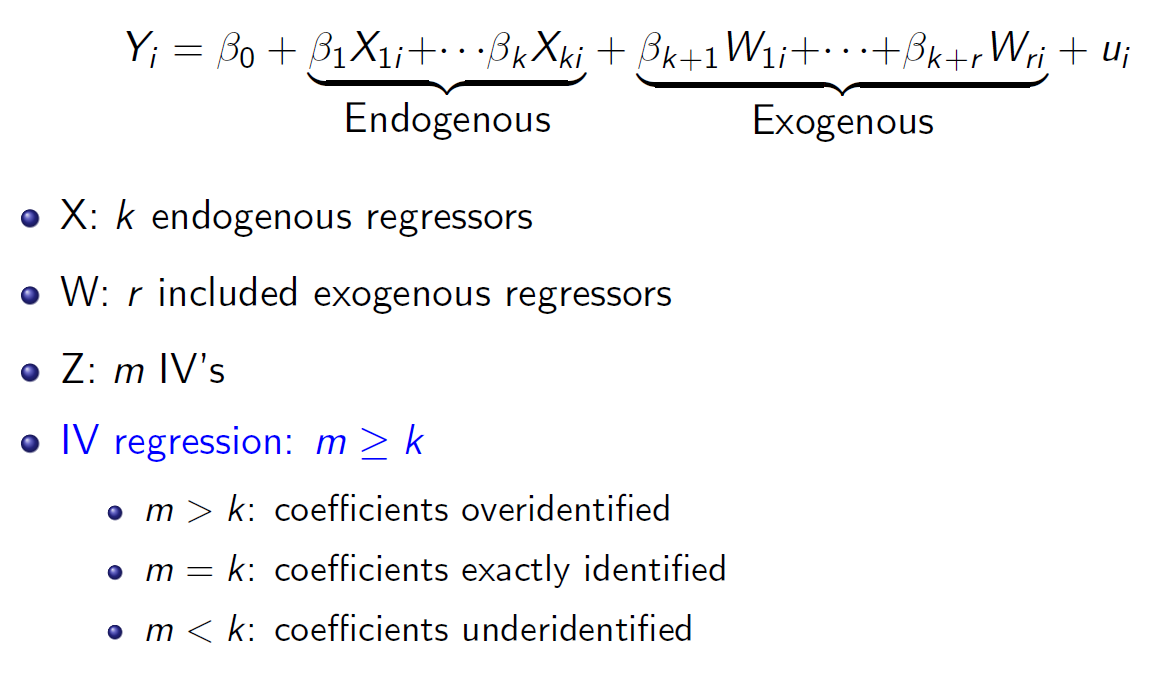
- overidentify & underidentify
- m = instrument 數
- k = endogenous regressor 數
- m < k → underidentified
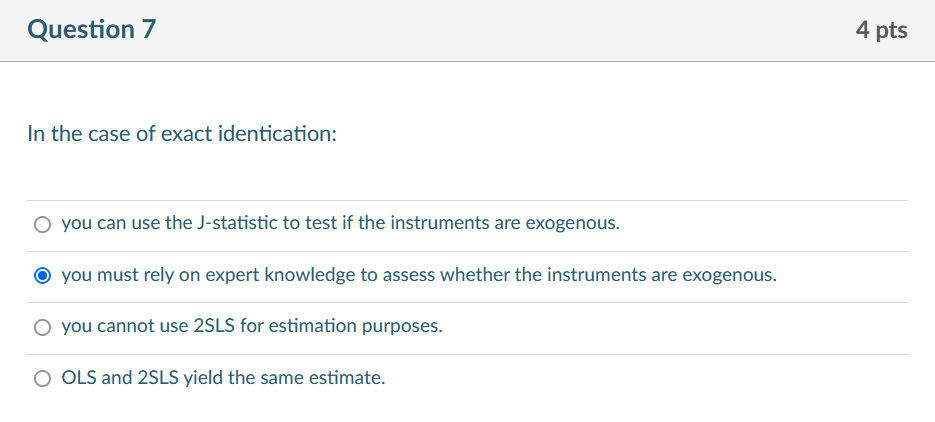
- m = k → exactly identified
- m > k → overidentified
- need m >= k for estimation of IV regression model
- 白話:有幾個跟 error term 有關的 variable,就需要有幾個 instrument
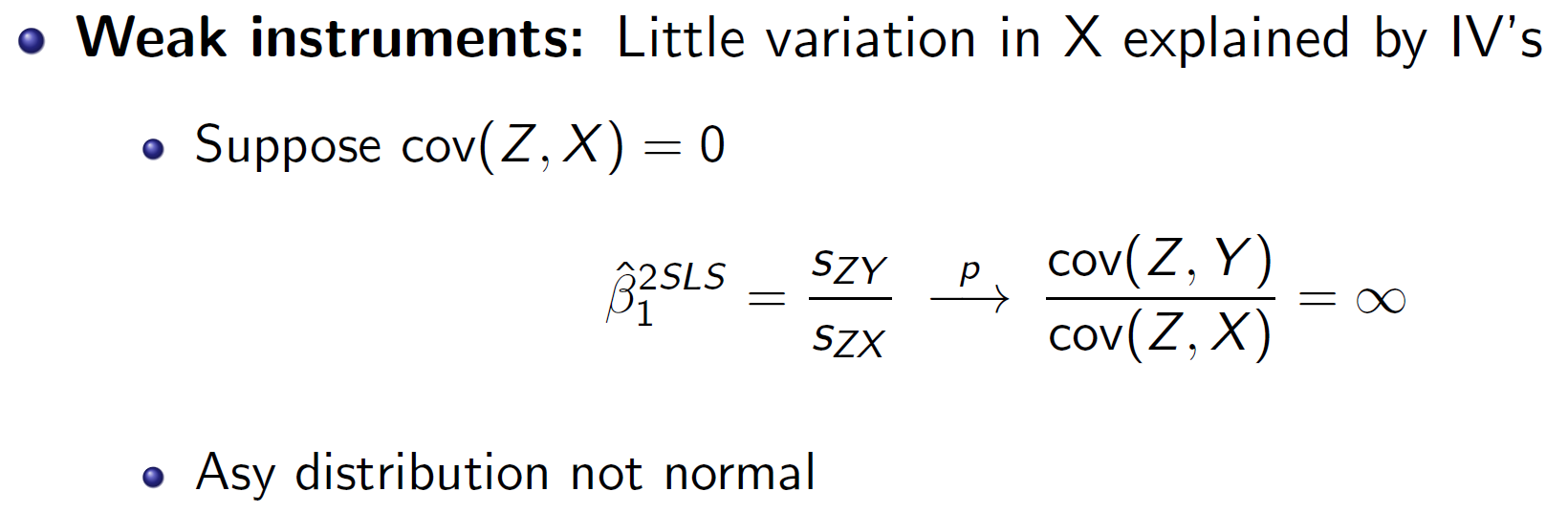
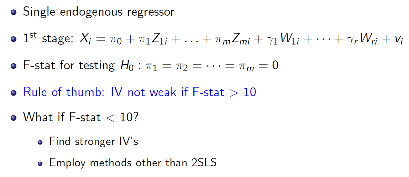
- weak
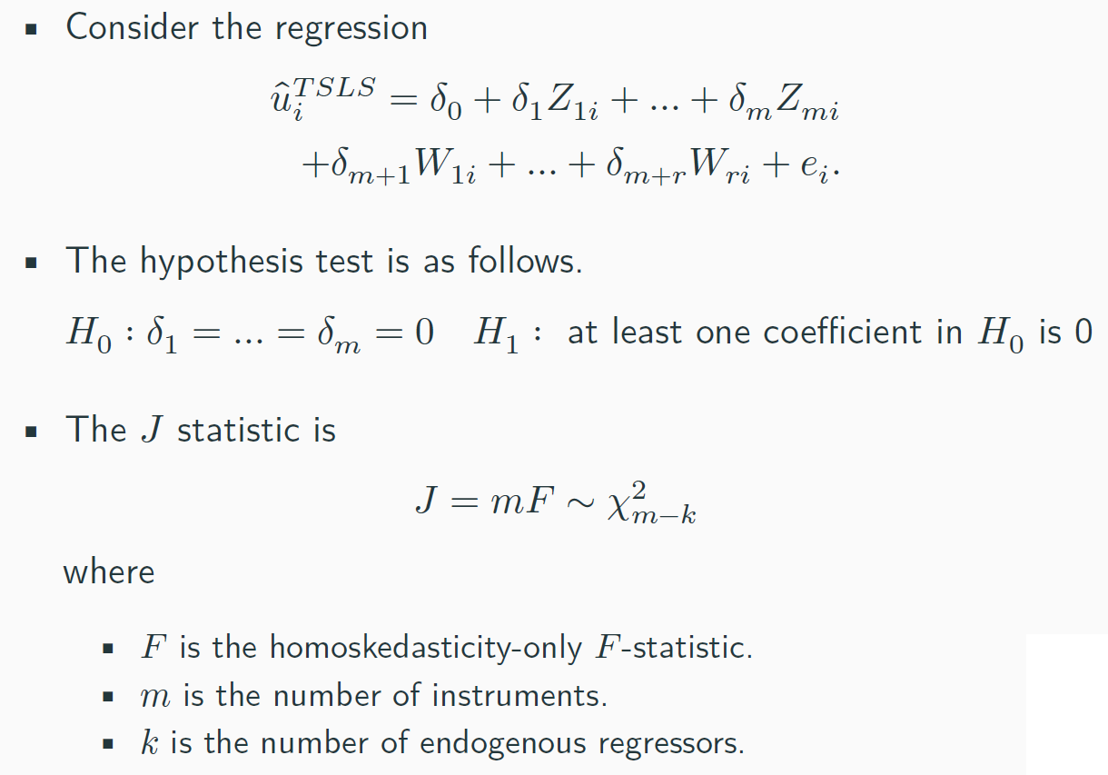
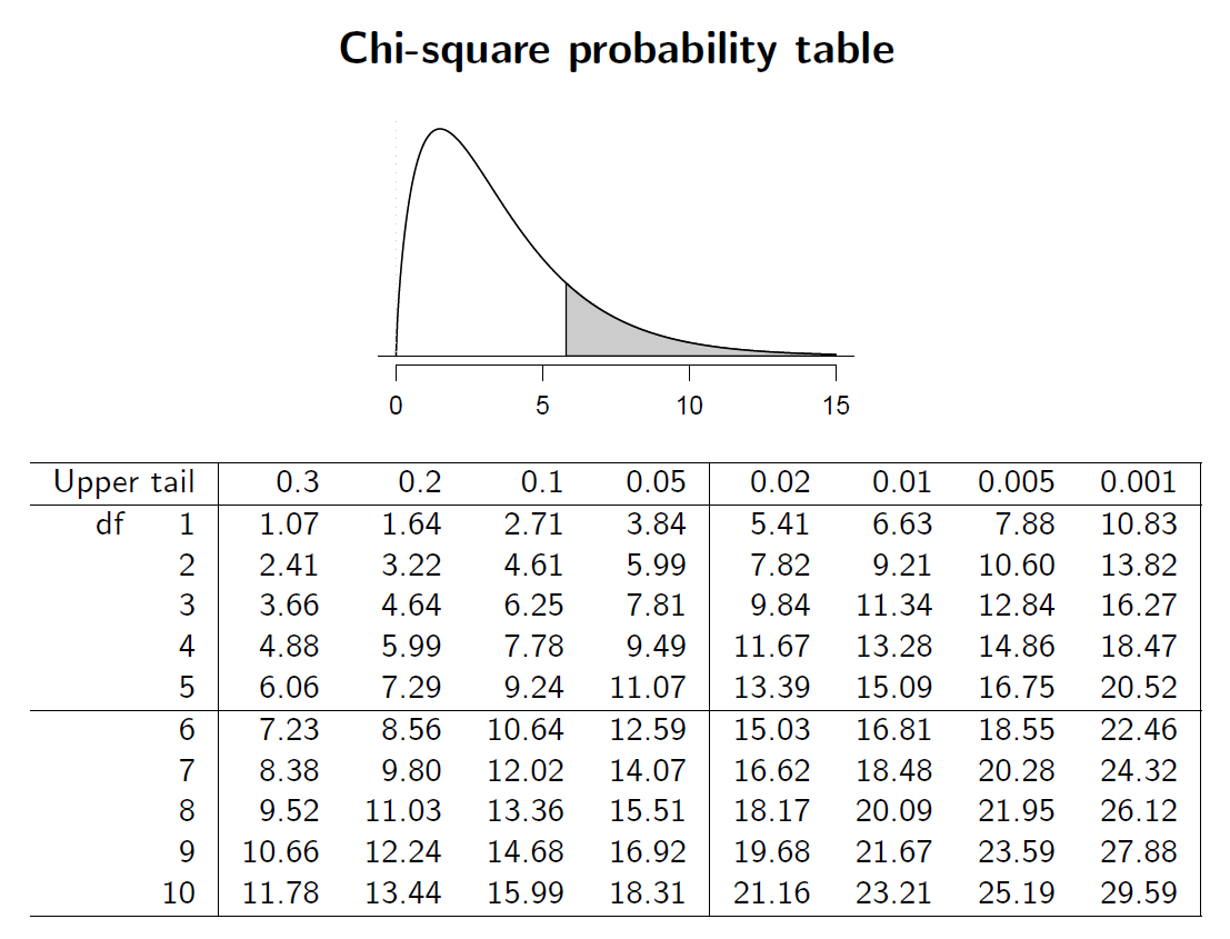
- overidentification test (J stat)
- test if if instrument is exogenous
- only possible to test this if overidentified
Ch13 Experiments & Quasi-Experiments
- differences-in-differences estimator
- treatment group 的平均改變 - control group 的平均改變
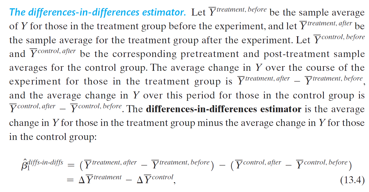
- t=1: before treatment
- t=2: after treatment
Ch14 big data
- 原始資料 notation:*
- OOS out-of-sample
- standardization
- prediction error = 實際 - 預測
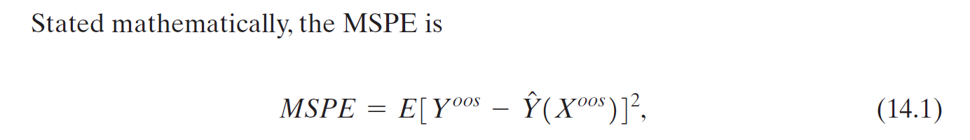
- MSPE min square prediction error
- expected prediction error when predicting for an observation out of the sample set
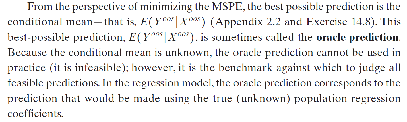
- oracle prediction
- prediction with smallest MSPE is conditional means
- no estimation error, only prediction error
- estimation error \(\sigma_\mu\)
- prediction error \(\sigma_u\) = variance of error term
- sparse model
- most predictors except some are 0
- shrinkage estimators
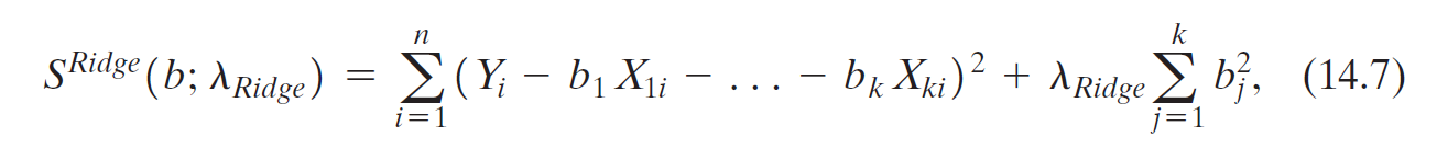
- Ridge
- Ridge
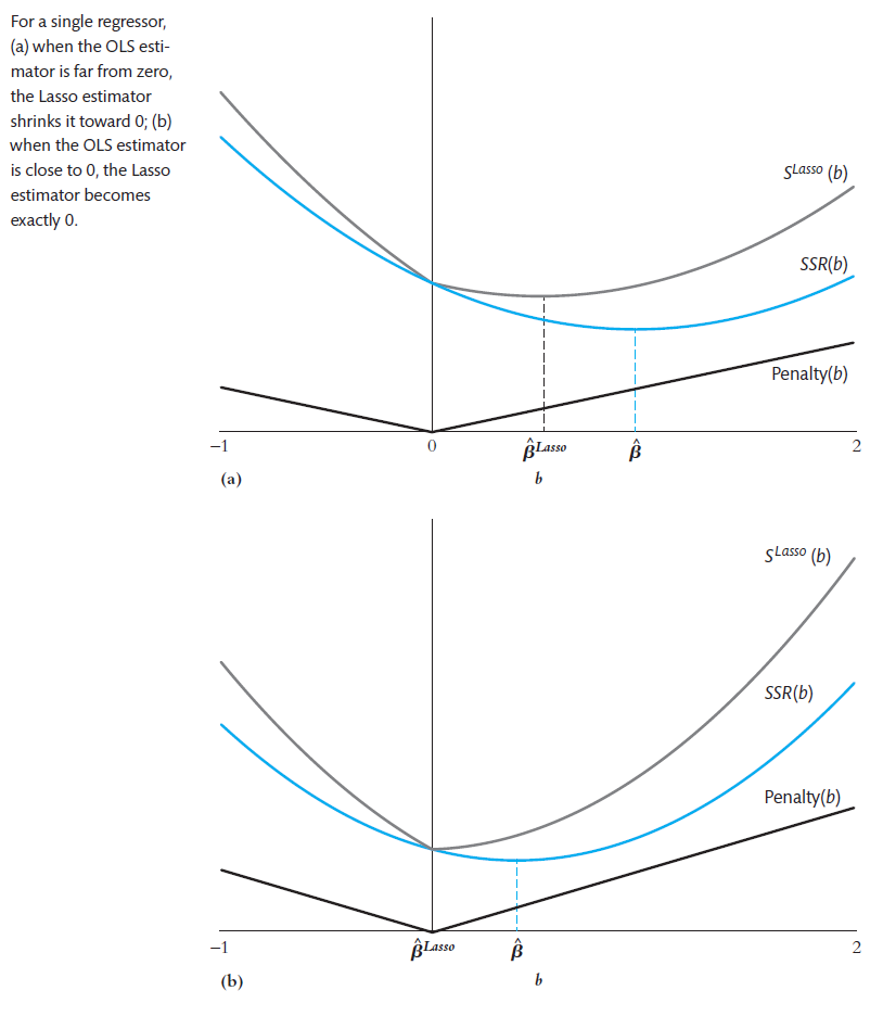
- Lasso
- least absolute shrinkage and selection operator
- set many estimators to be 0
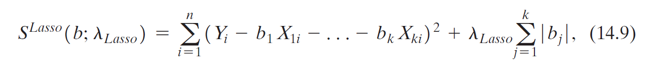
- \(\lambda_{Lasso}\): Lasso shrinkage parameter
- \(\hat{\beta}^{Lasso}\) Lasso estimator = value of \(b\) to minimize \(S^{Lasso}(b;\lambda_{Lasso})\)
- penalty term (second term): penalize large \(b\), shrinking Lasso estimate toward 0