Machine Learning

resources

• course website
• github

training techniques

gradient accumulation

to avoid CUDA out of memory problem

e.g. batch size = 8 -> batch size = 2 but accumulate 4 iterations before optimizing

for at each iteration

loss /= accum_iter
if ((batch_idx + 1) % accum_iter == 0) or (batch_idx + 1 == len(data_loader)):
    optimizer.step()
    optimizer.zero_grad()

https://kozodoi.me/python/deep%20learning/pytorch/tutorial/2021/02/19/gradient-accumulation.html

intro

• gradient decsent
  • 
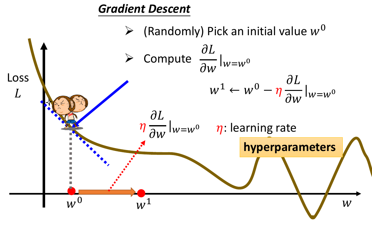
  • 微分取斜率
  • 往左/右走多少 depends on 斜率
  • 卡在 critical point (微分 = 0)
    • local minima or saddle point
• sigmoid function
  • sigmoid(f(x)) = \(e^{f(x)}\)
  • 
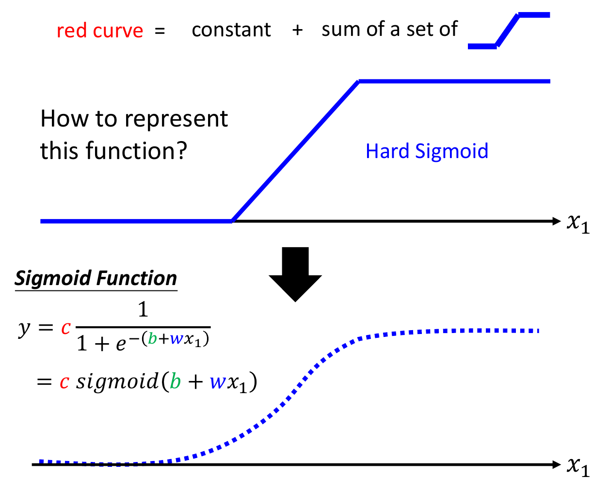
  • 疊加一堆 sigmoid 逼近 function
• hyperparameter
  • 你自己設的 parameter
• deep learning
  • 堆很多層 ReLU
  • 很多層 -> overfitting

general guidance

• improving your model
  • training loss big
    • deeper network has bigger loss
      • optimization problem
    • model bias
      • make model bigger, more complex
  • training loss small. testing loss big
    • overfitting

overfitting

• 
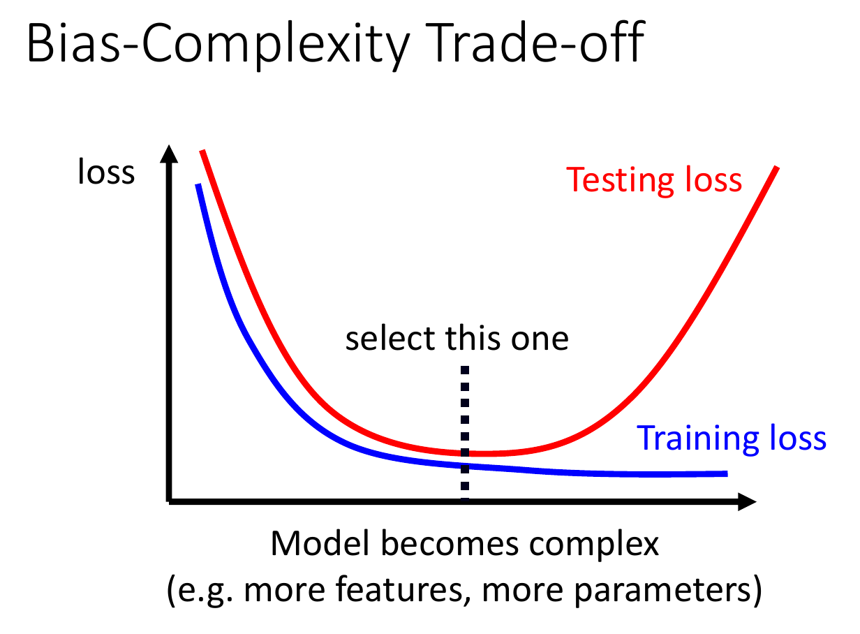
• to solve
  • less parameters
  • less features
  • early stopping
  • regularization
  • dropout
  • weight decay
    • to limit the freedom of your model

critical point

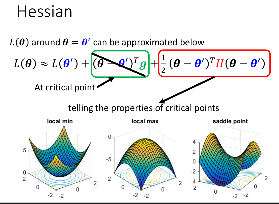
• eigen value all positive -> local minima
• eigen value all negatuve -> local maxima
• eigen value 有正有負 -> saddle points

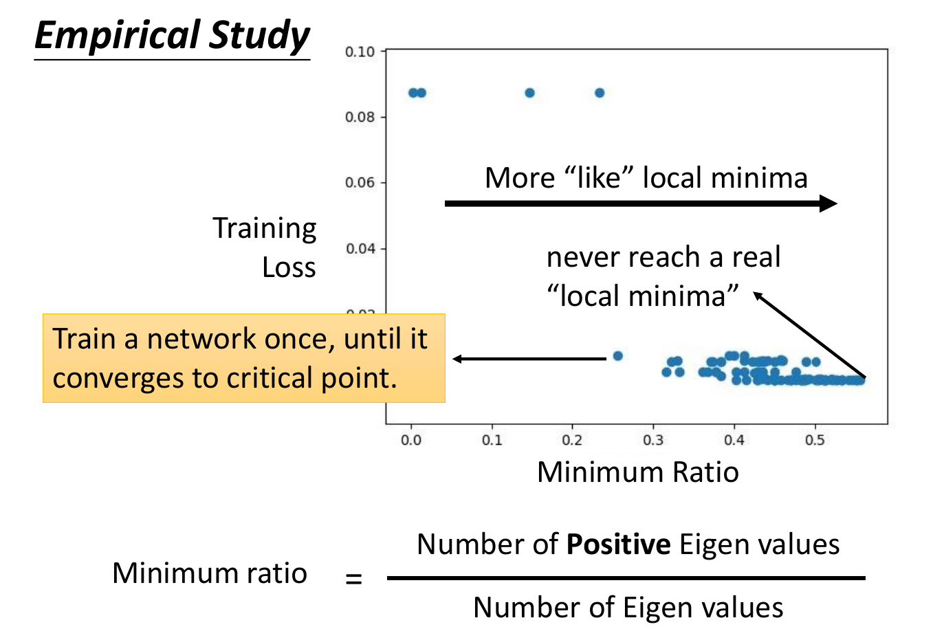表示大部分時候都不是卡在 local minima，而是 saddle point

gradient descent 事實上很少卡在 critical point，而是在附近震盪 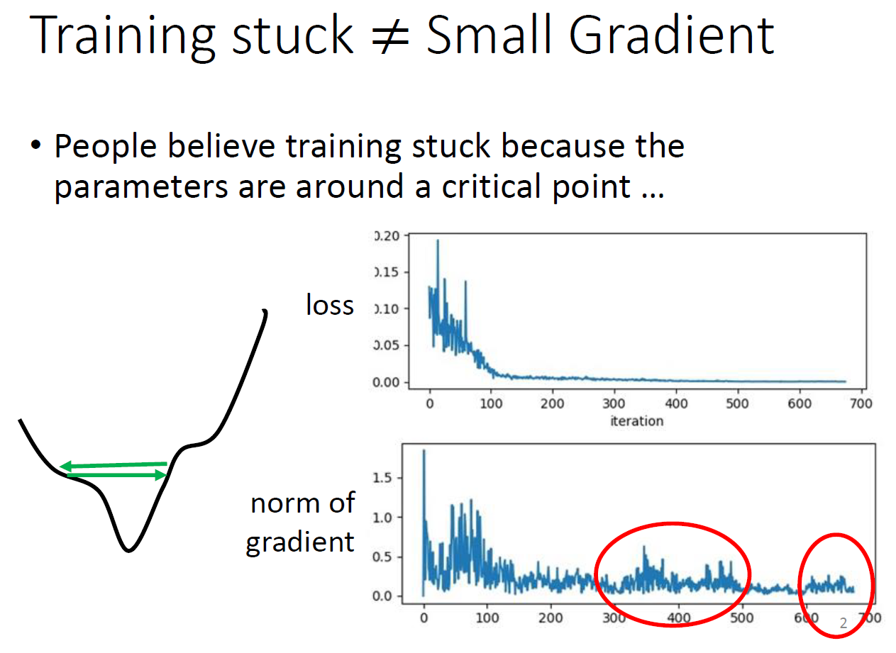要達到 critical point 要用特殊的方法

batch

• epoch
  • see all batches i.e. all data in a batch
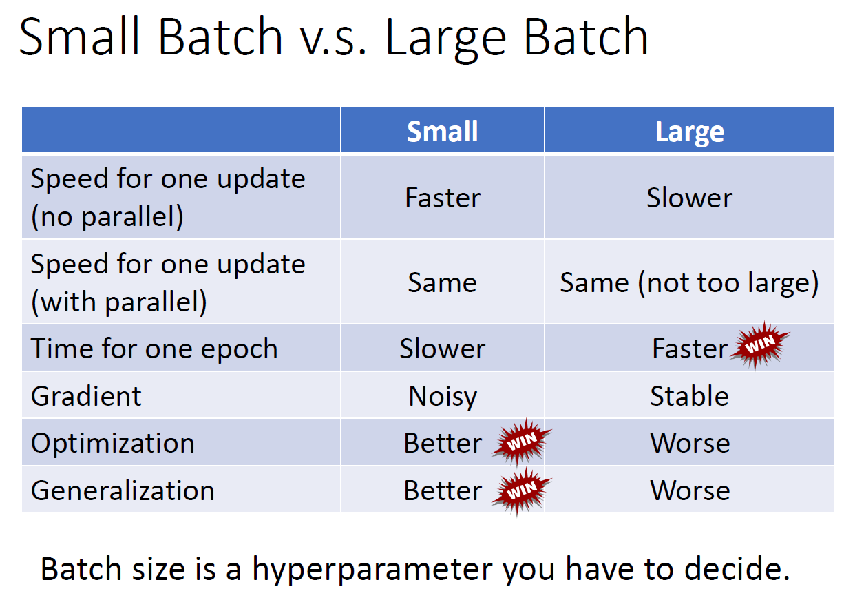
• small batch
  • see few data in a batch
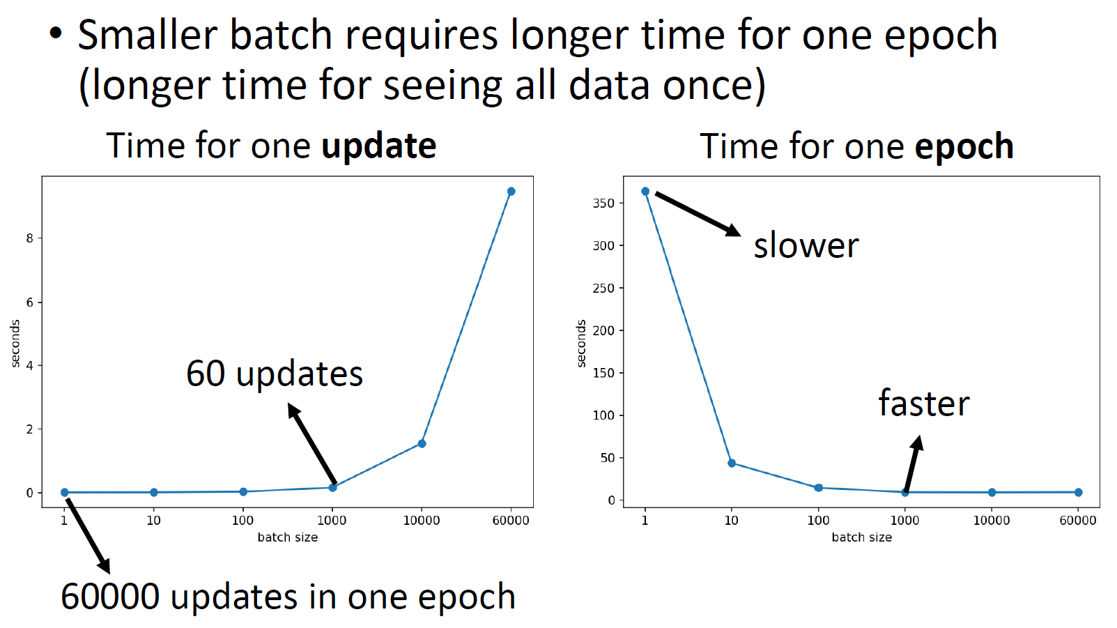
  • more batch in an epoch
  • can use parallel computing in a batch -> not necessarily bigger epoch time
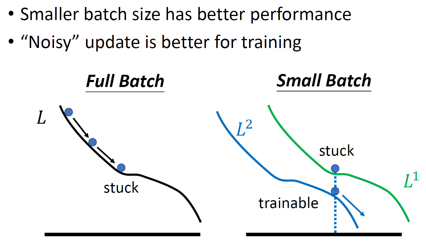
  • updates more noisy
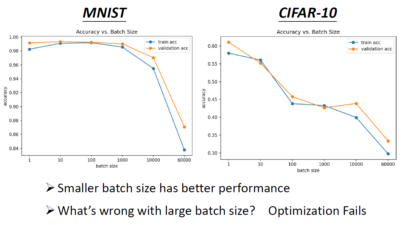
    • loss function different for each batch -> more noisy -> less likely to fall into local minima -> better training accuracy
      • 
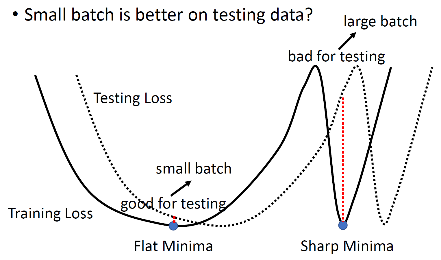
    • tends to fall more in flat local minima than in sharp local minima -> better testing accuracy
      • flat local minima is better than sharp local minima
      • 
• big batch
  • see many data in a batch
  • less batch in an epoch
  • less epoch time
  • less training accuracy
  • less testing accuracy
• big batch size -> less epoch time
  • 
• big batch size -> less training accuracy
  • 
• 

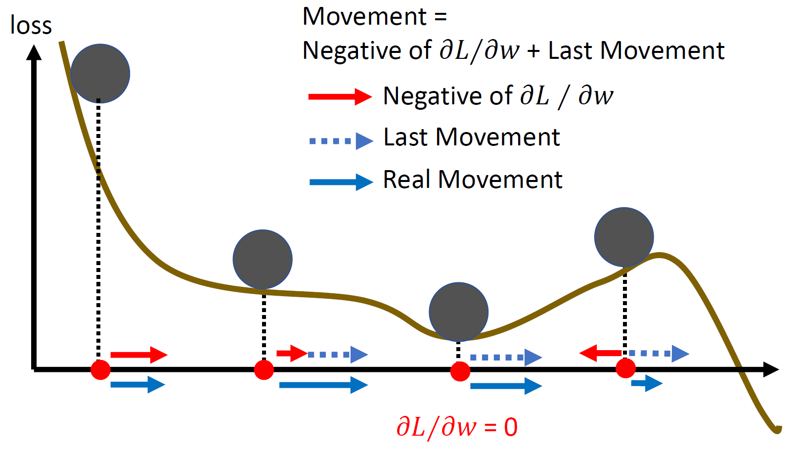
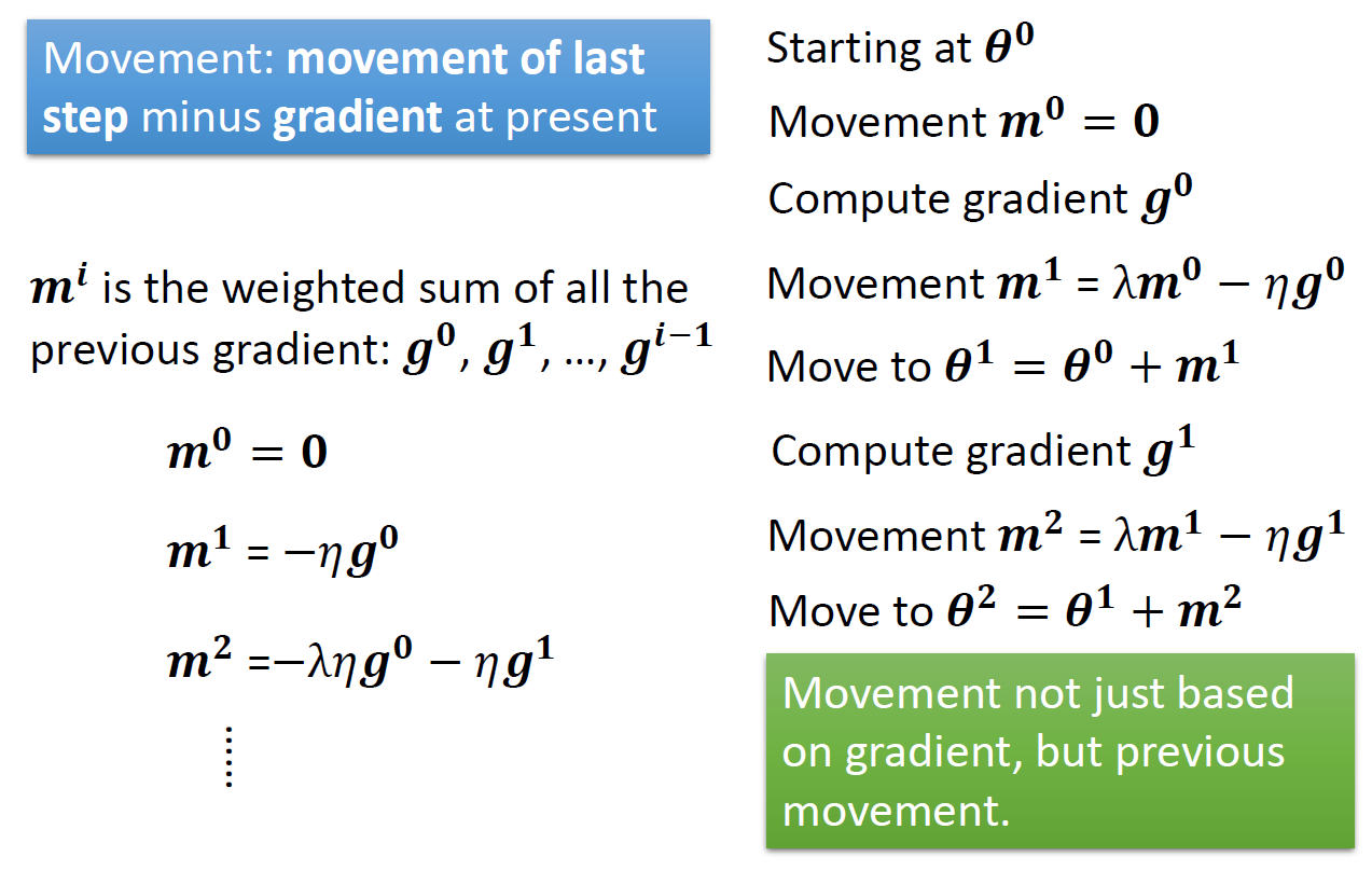
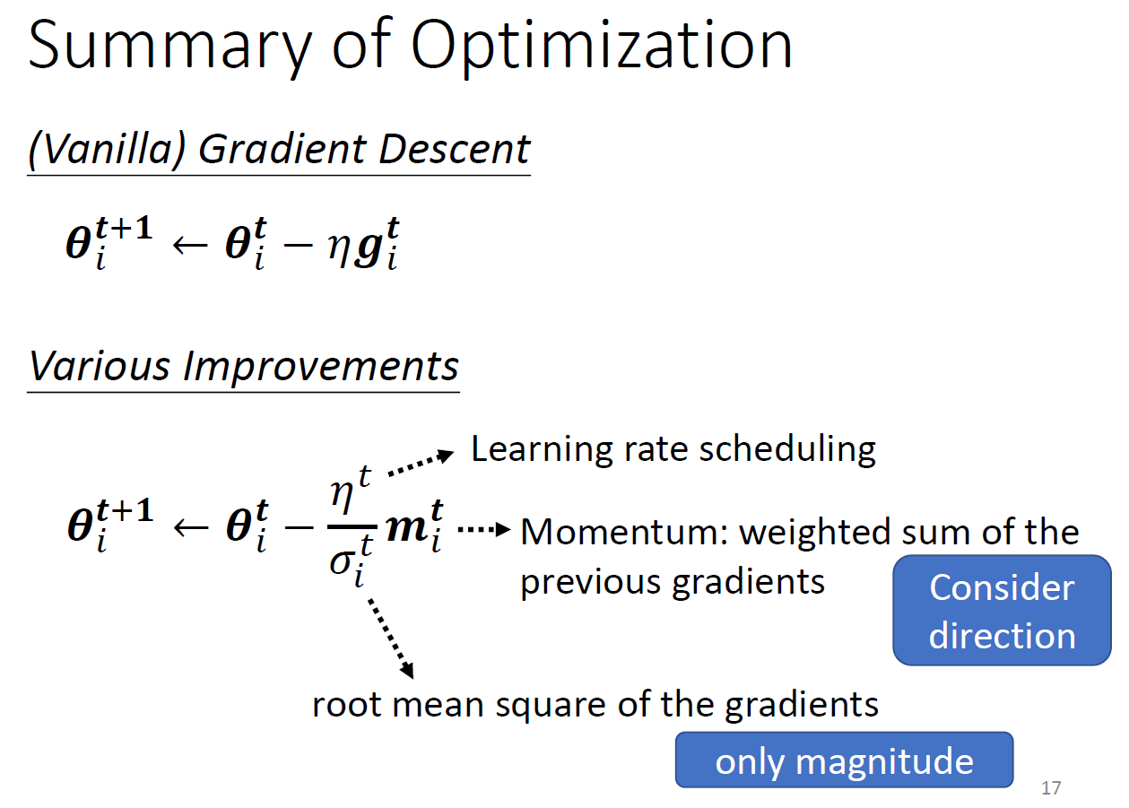
momemtum

• 
• 
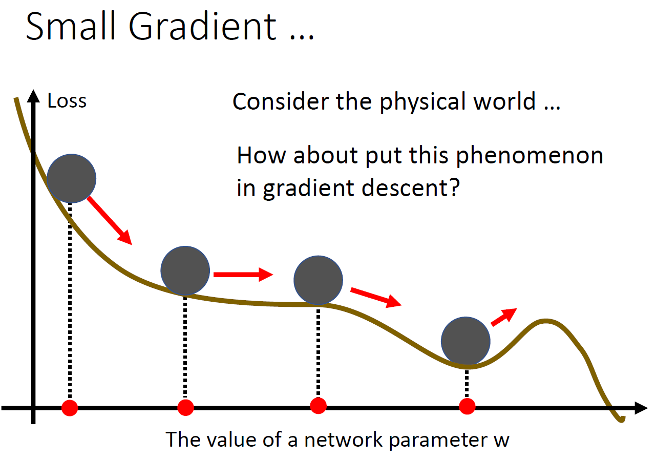
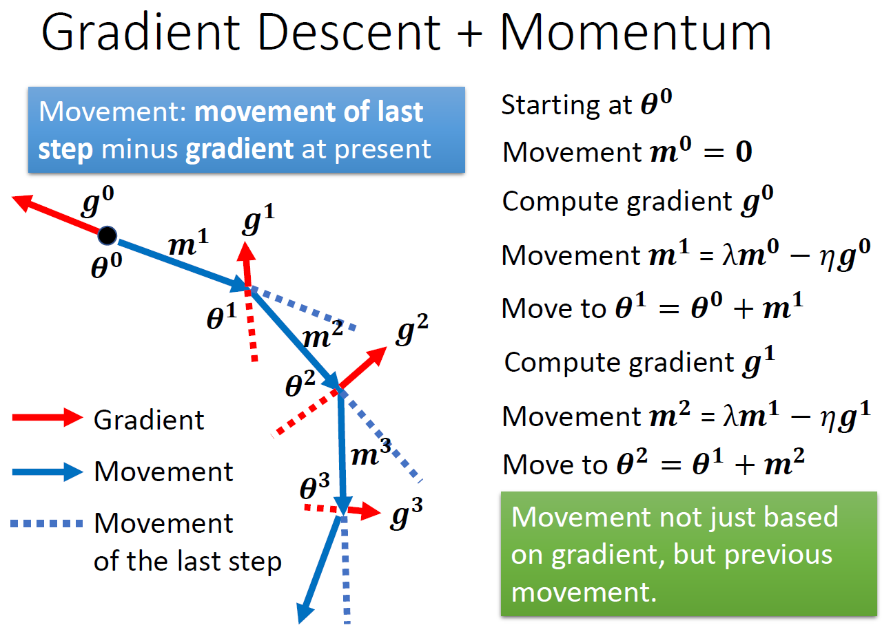
• momemtum = weighted sum of all previous gradients
  • 
• 

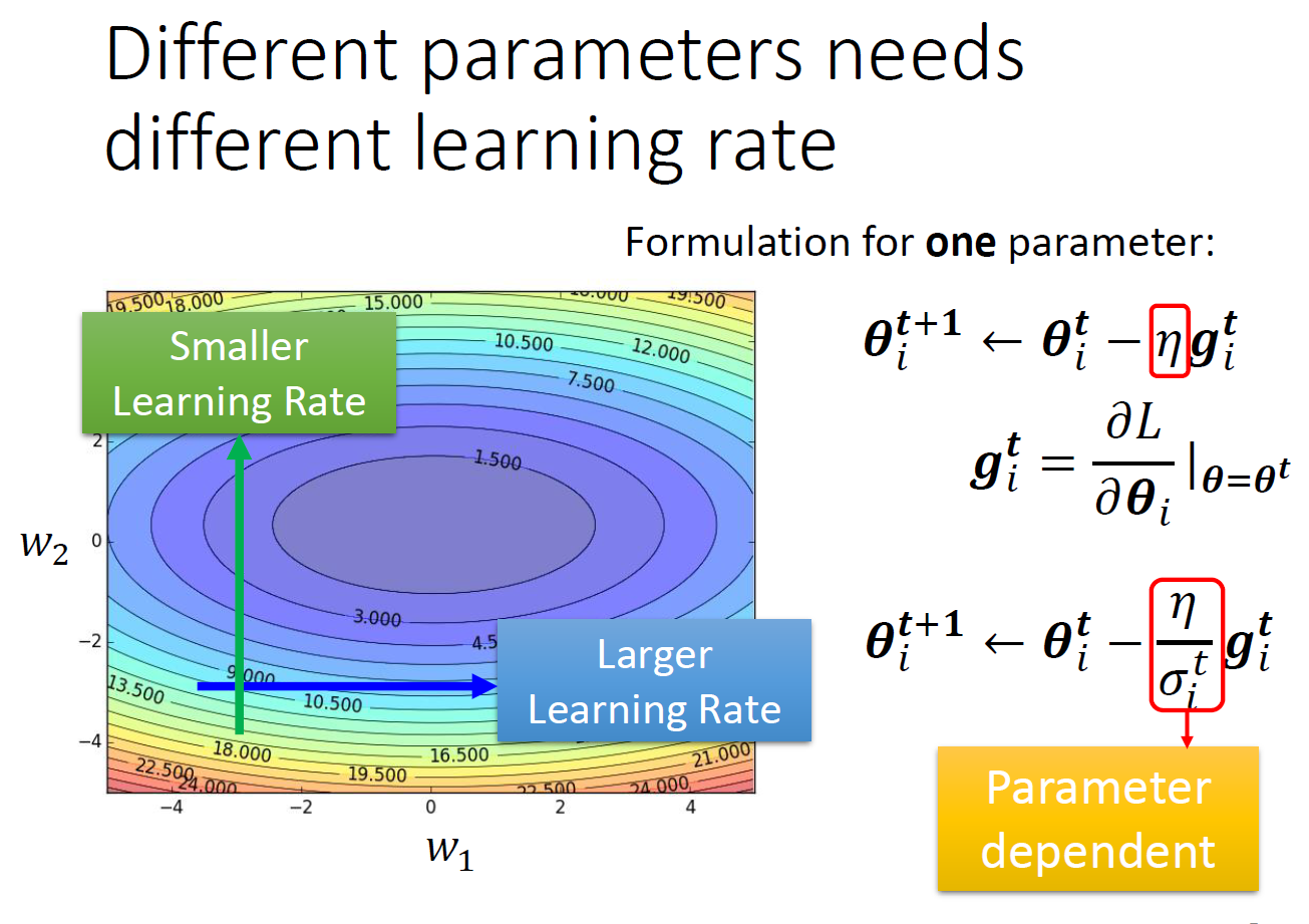
adaptive learning rate (optimization)

• learning rate = 步伐大小
• small slope -> big learning rate
• big slope -> small learning rate
• 
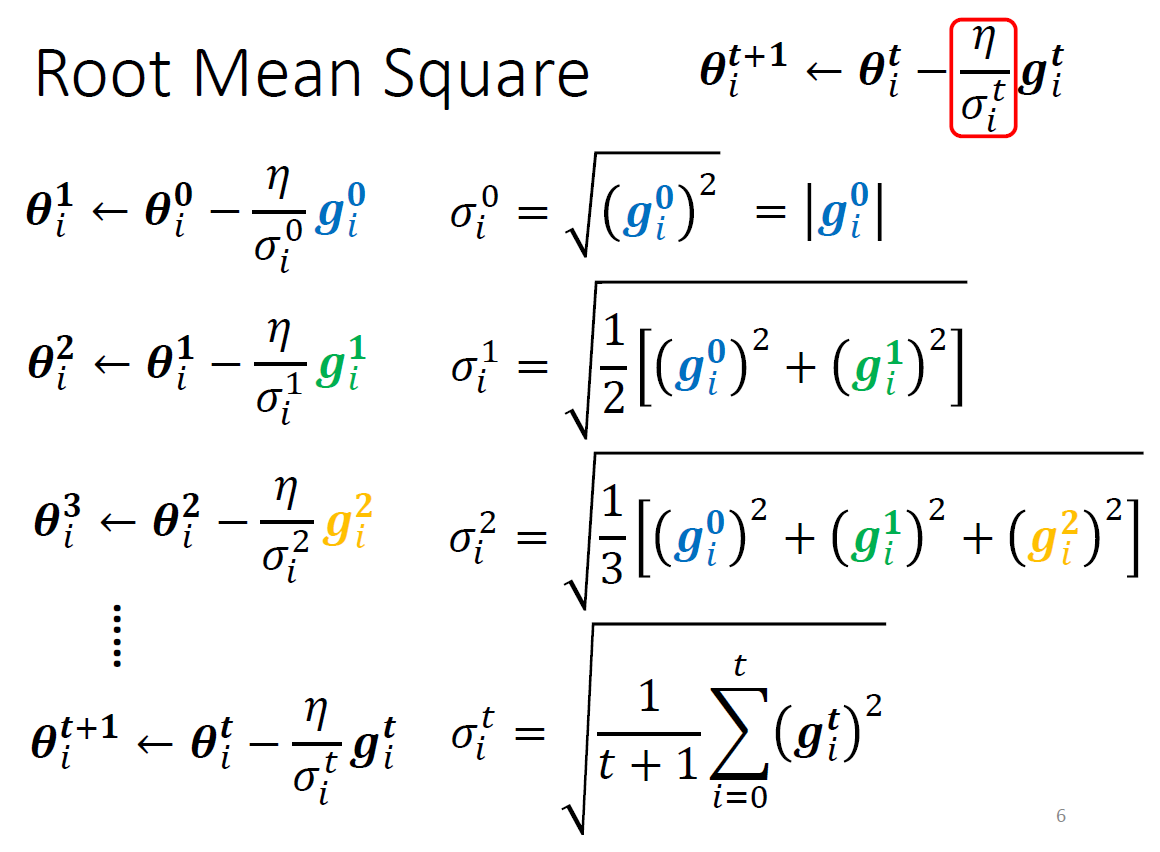
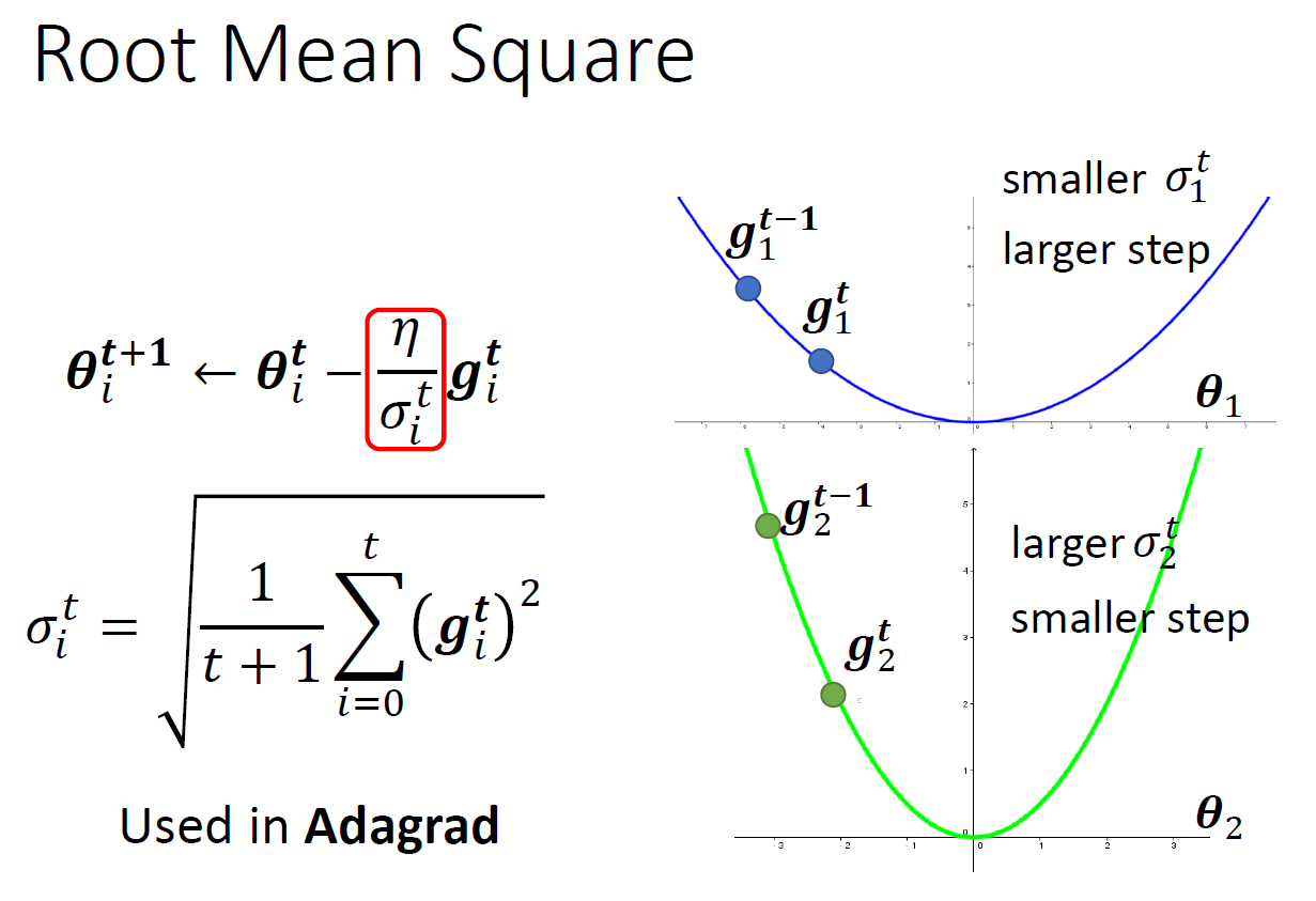
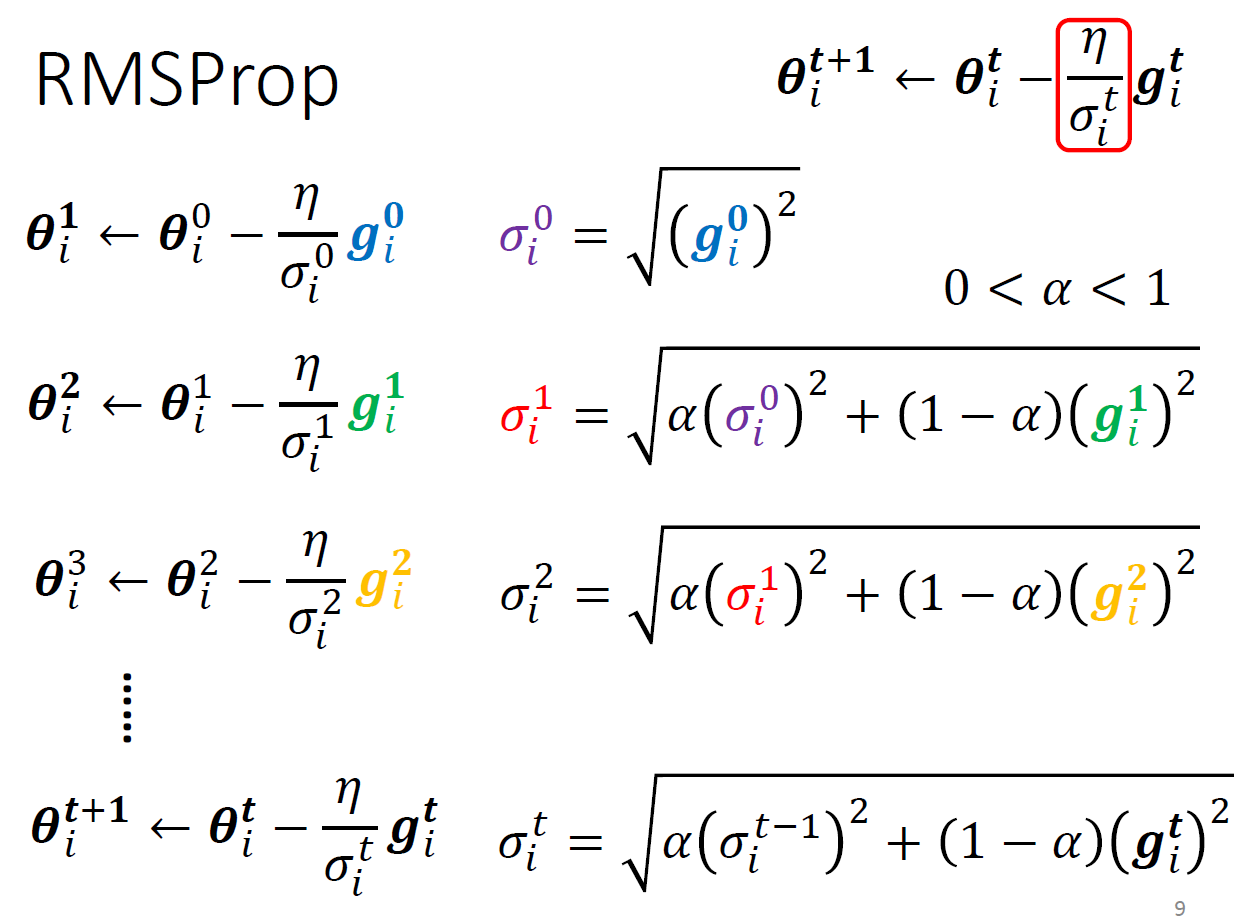
• using RMS
• Adagrad
• g small -> \(\sigma\) small -> learning rate big
• 把過去所有 gradient 拿來取 RMS
• calculation
• 
• 
• gradient 很小 -> \(\sigma\) 很小 -> 在平坦的地方爆出去
• 
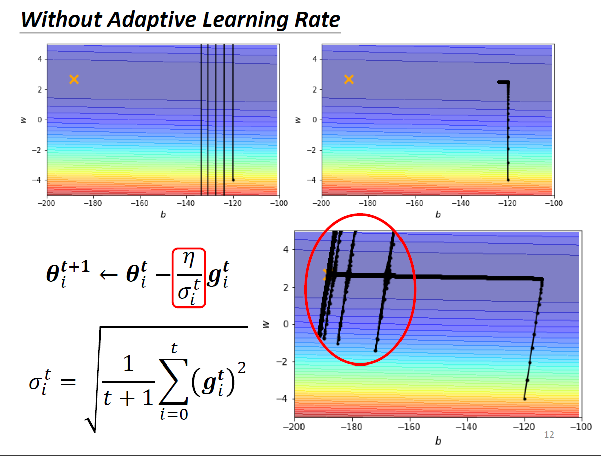
• to improve
• 
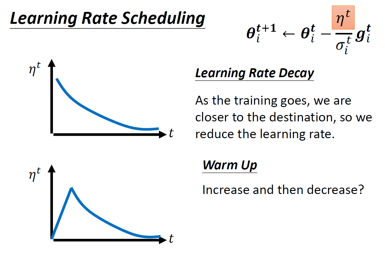
• warm up
  • 先用小 learning rate 探索 error surface
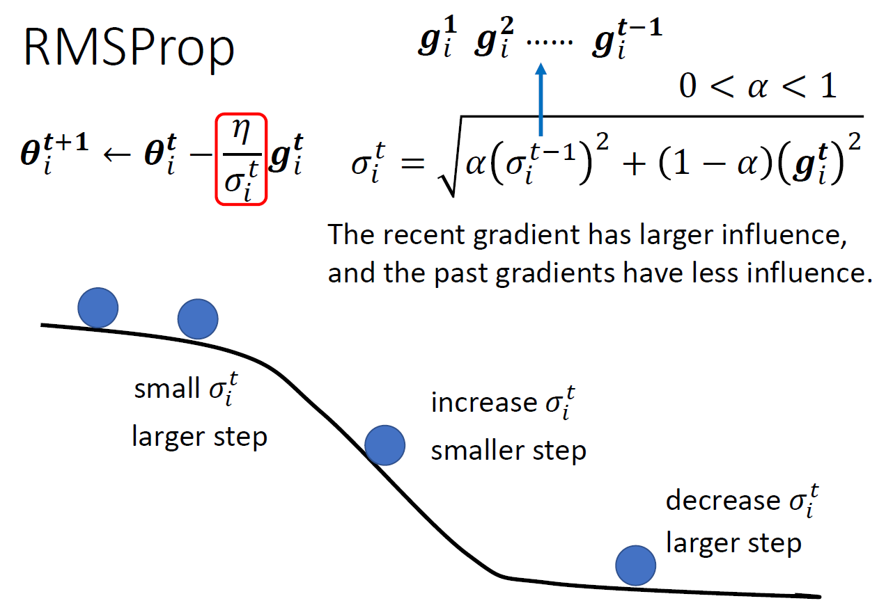
• using RMSProp
  • no original paper
  • Adam: RMSProp + momemtum
  • set, \(\alpha\), weight of current gradient, by yourself
  • current gradient is more important (like EWMA)
  • calculation
    • 
    • 
• 

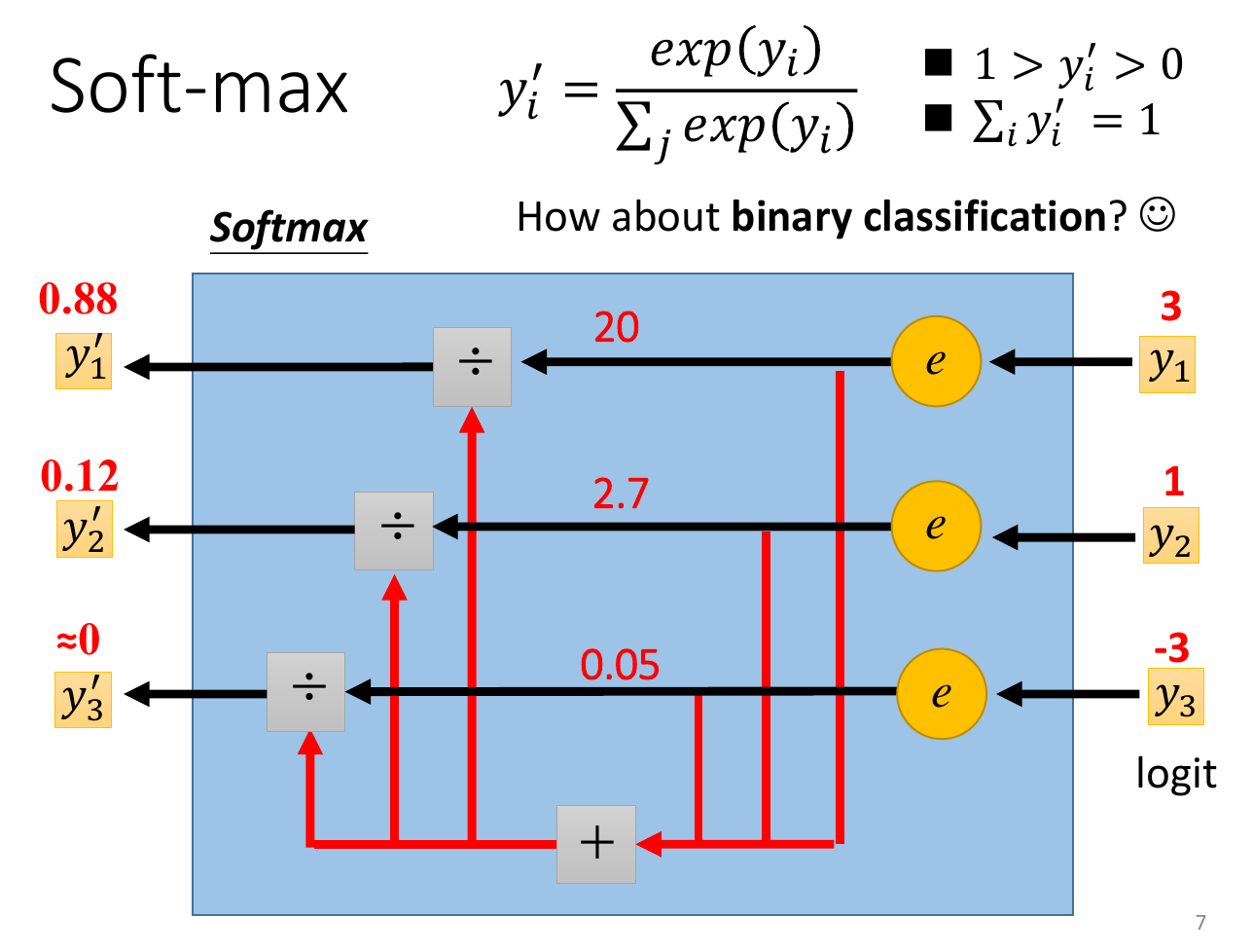
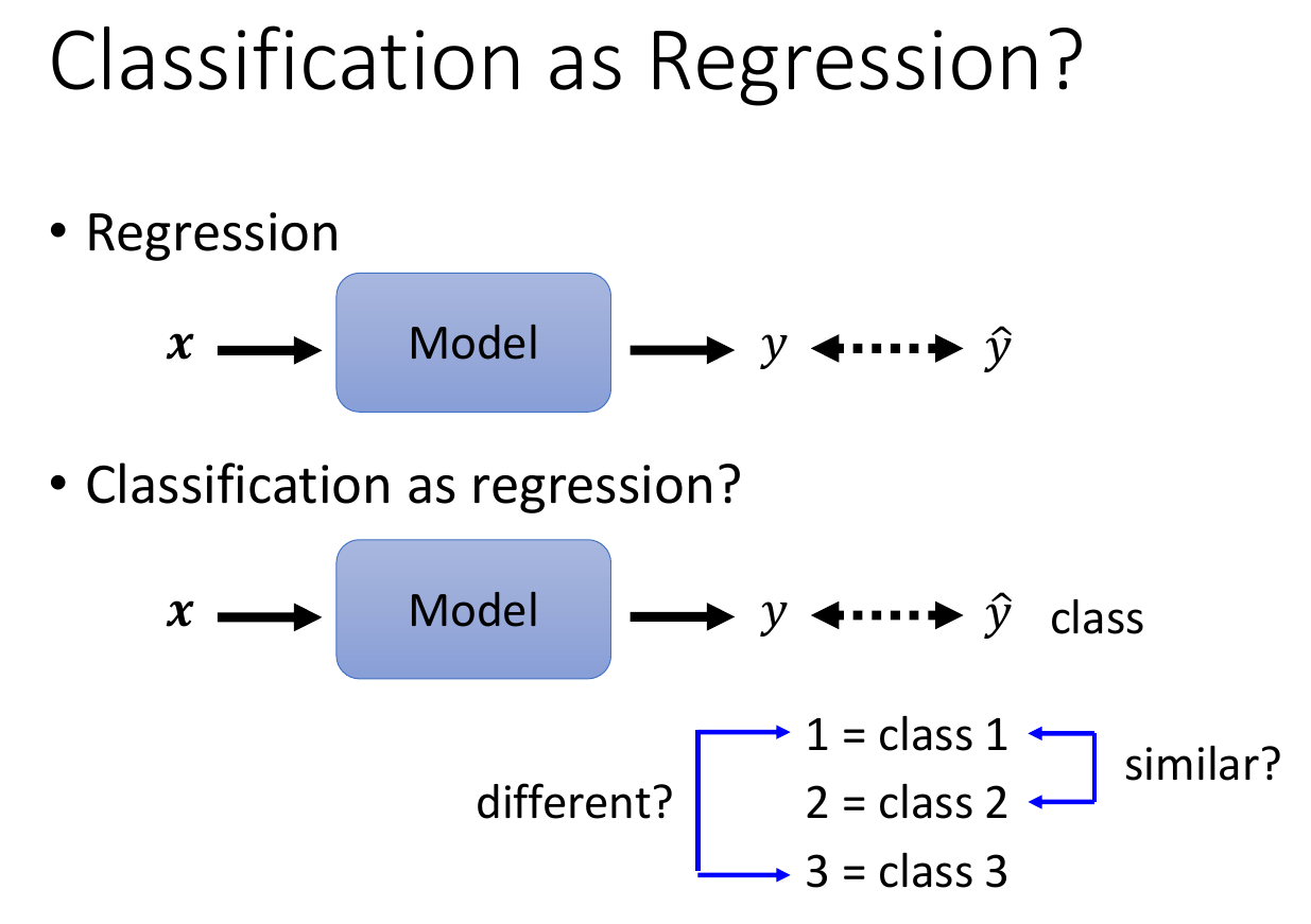
classification

• 希望 model output 接近 class 的值
  • 
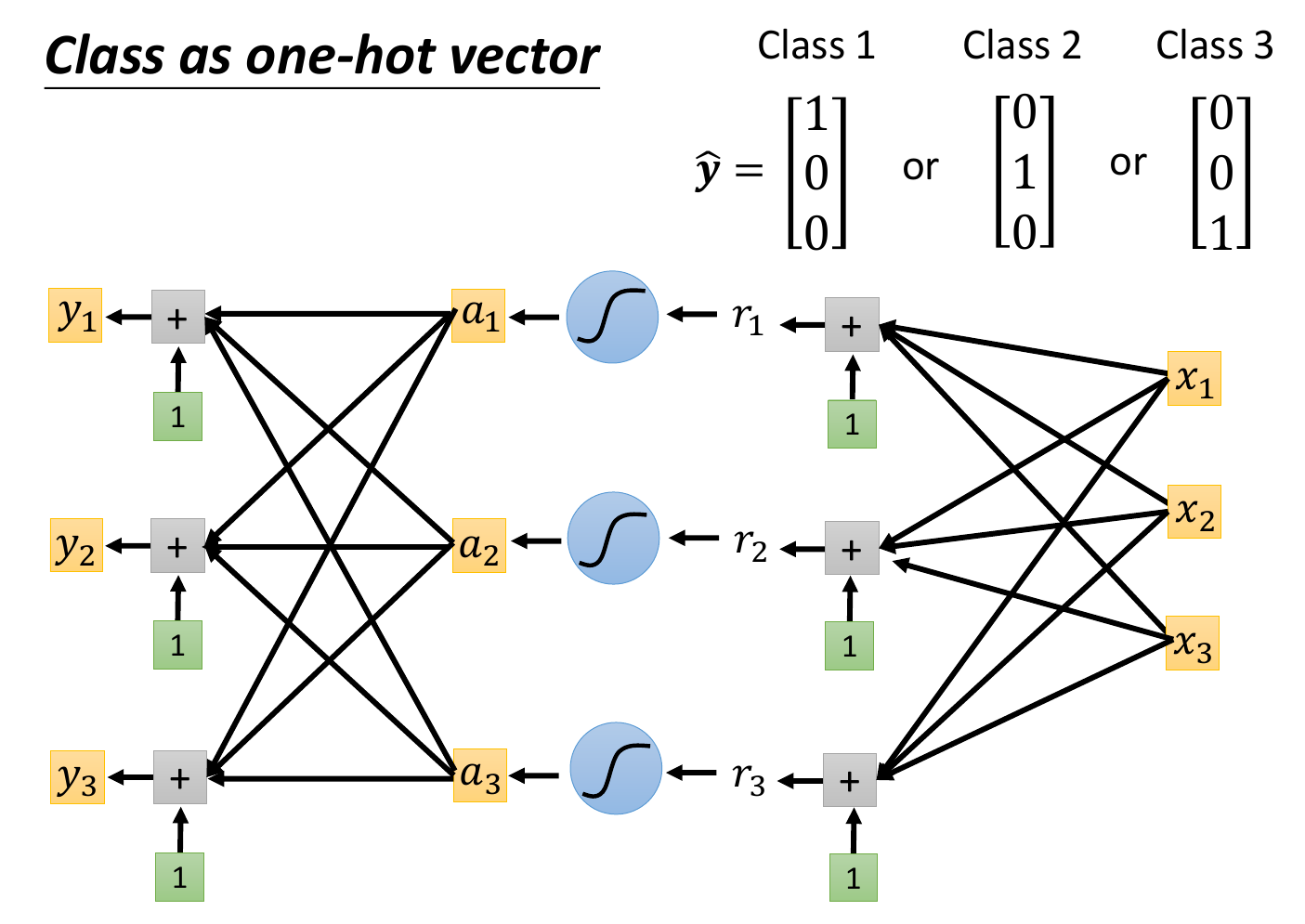
• represent class as one-hop vector (binary variable)
  • 
• softmax
  • nomalize to 0-1
  • 

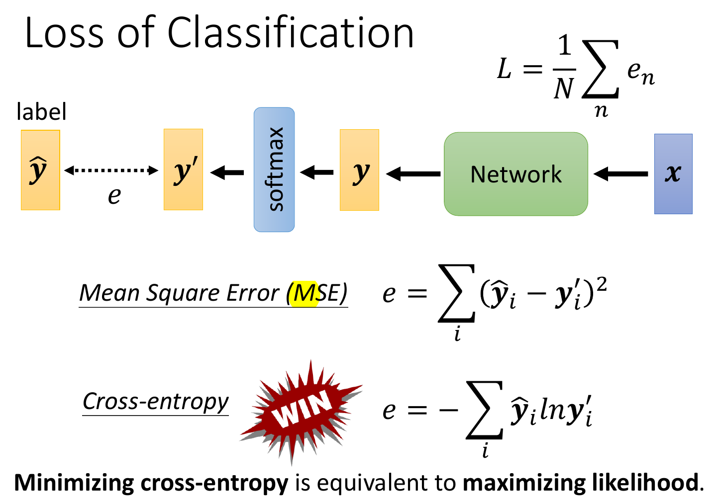
loss

• MSE
• cross entropy
  • minimize cross entropy = maximize likelihood
  • pytorch cross entropy includes softmax already
  • better than MSE
    • easier for optimization
      • ]
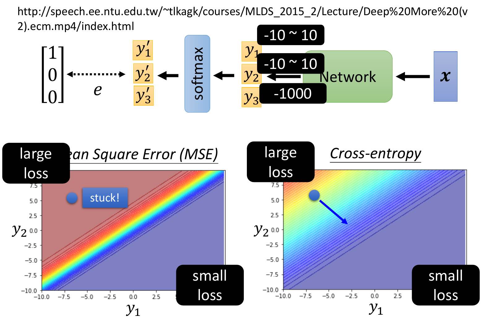      • with MSE, when start at left top (y1 small, y2 big, loss big), slope = 0 -> can't use gradient descent to reach right bottom (y1 big, y2 small, loss small)
• 
• BCEWithLogitsLoss with pos_weight for imbalanced dataset

ROC & AUC Curve

• For balanced dataset
• ROC curve
  • true positive rate vs. false positive rate under different threshold
  • 
• AUC Curve
  • Area under ROC curve

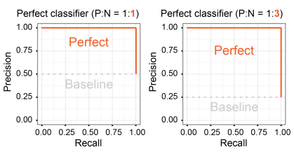
Precision Recall Rate

• For imbalanced dataset
• Precision vs. Recall Rate under different threshold
• 

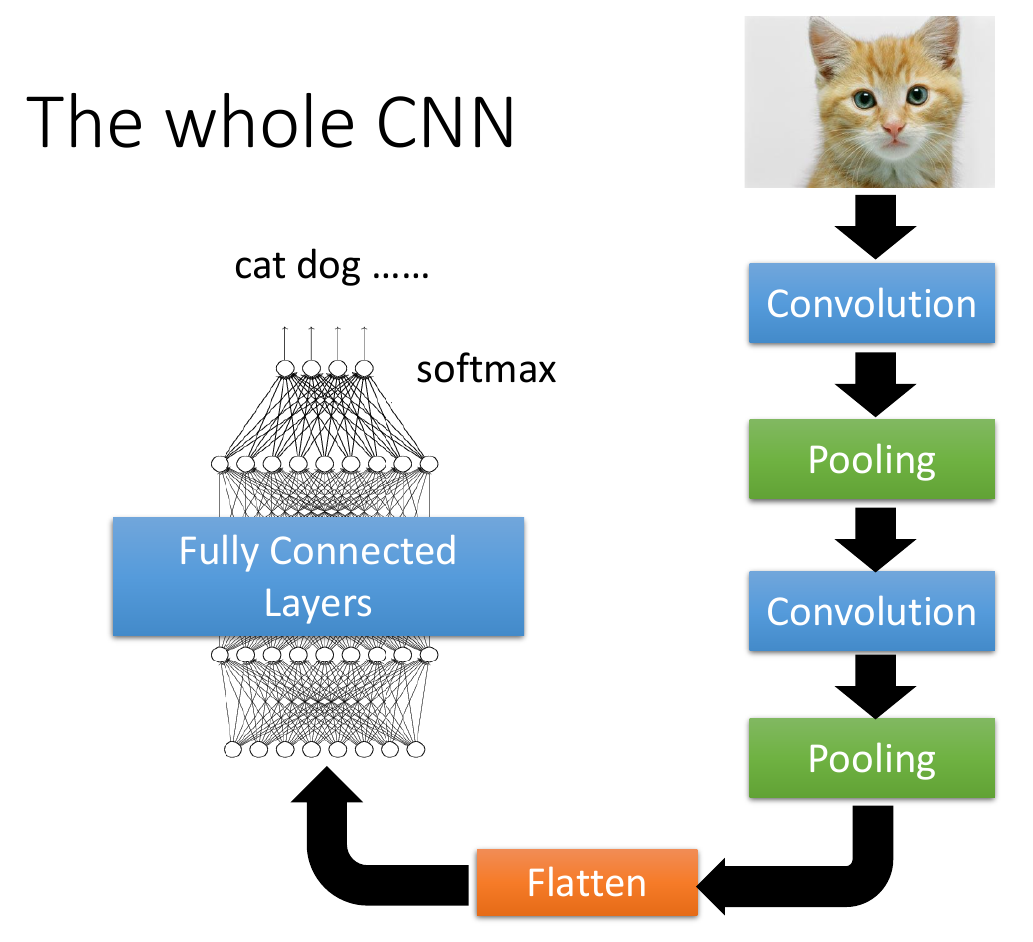
CNN

• image classification
  • 3D tensor
    • length
    • width
    • channels
      • RGB
  • convert 3D tensor to 1D vector as input
• 
• alpha go
  • 下圍棋: 19x19 (棋盤格子數) classification problem
  • treat 棋盤 as an image and use CNN
  • 格子 = pixel
  • 49 channels in each pixel
    • to store the status of the 格子
  • 5x5 filter
  • no pooling
• intolerant to scaling & rotation
  • to solve
    • data augmentation
      • rotate and scale first to let CNN know
    • spatial transformer layer

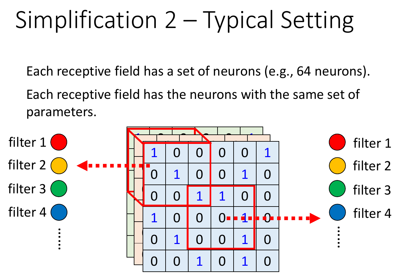
receptive field

• each neuron has a part as input, instead of giving in the whole image
• 
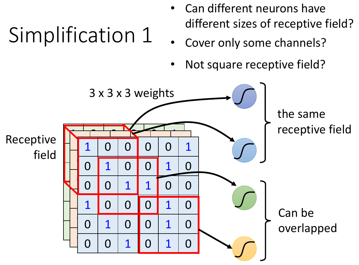
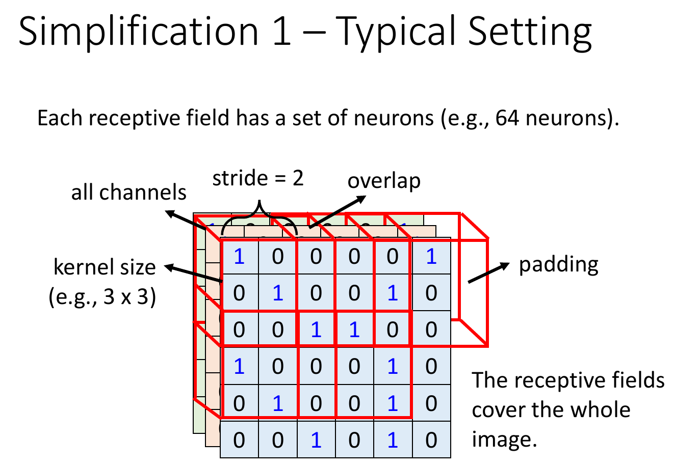
• typical settings
  • kernel size = 3x3 (length x width)
  • each receptive field has a set of neurons
  • each receptive field overlaps
    • s.t. otherwise things at the border can't be detected
  • stride = the step, the distance between 2 receptive field
  • when receptive field is over the image border, do padding i.e. filling values e.g. 0s -> zero padding
  • 

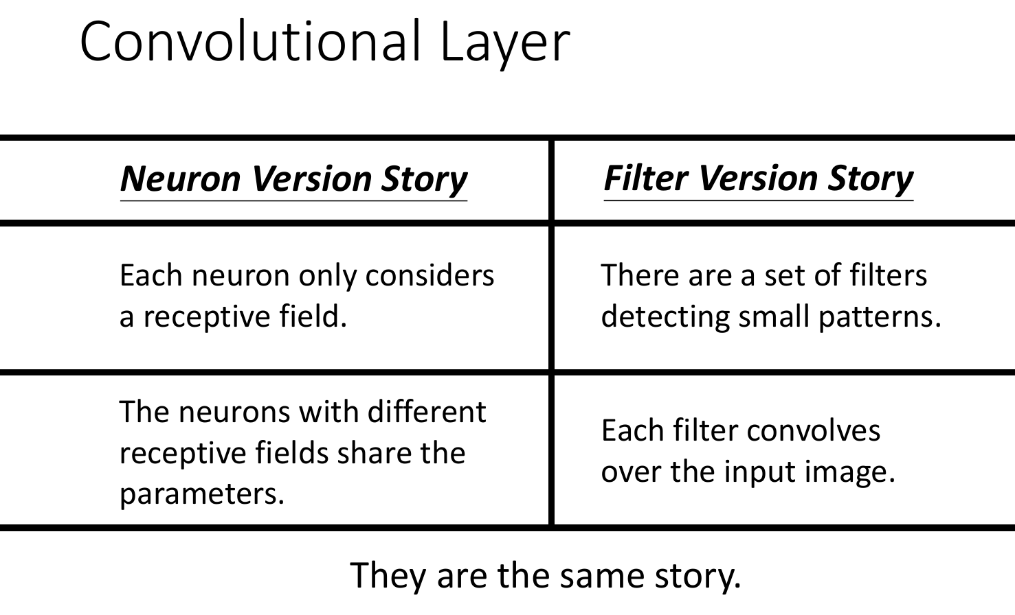
filter

• parameter sharing
  • having dedicated neuron (e.g. identifying bird beak) at each receptive field is kind of a waste -> parameter sharing
  • same weight
• filter
  • a set of weight
  • used to identify certain patterns
  • do inner product with receptive field -> feature map, then find fields giving big numbers
    • 
    • 
• 
• typical settings
  • 

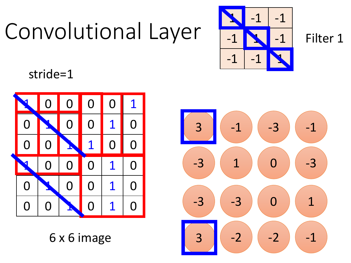
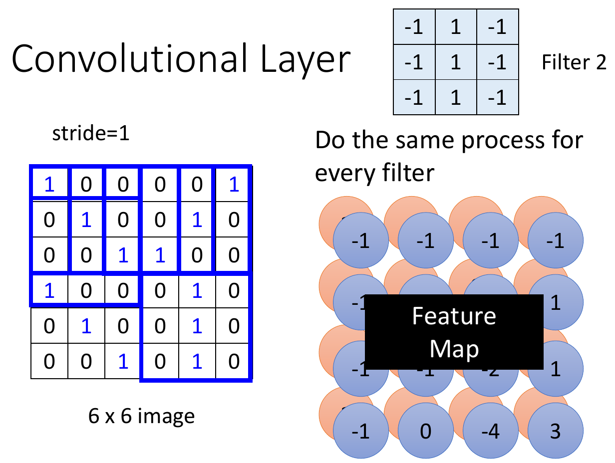
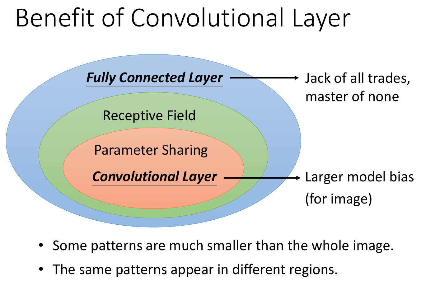
convolution layer

• fully connected
  • complete flexibility
  • can look at whole or only a small part
• receptive field
  • lower flexibility
  • limited to only look at a small part
• parameter sharing
  • lowest flexibility
  • forced to use shared parameters
  • convolution layer
  • bigger bias
    • good for specific tasks e.g. image classification
• 
• neural network using convolutional layer -> CNN

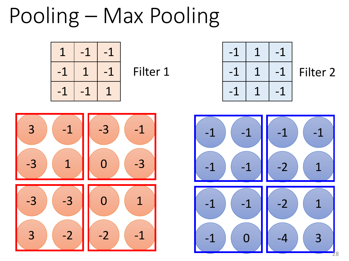
pooling

• subsampling, make image smaller
• to reduce computation
  • have enought compulation resource -> can omit pooling
• max-pooling
  • only select the larger number after applying filter
  • 

self attention

• input a (set of) vector(s)
  • 
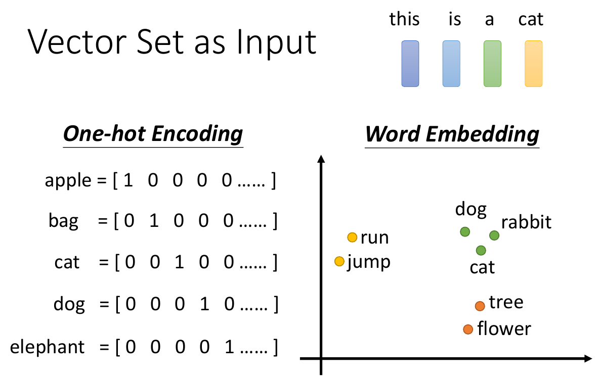
  • one-hot vector cons
    • treat each as independent, but there may be some correlations for some
  • graph -> a set of vectors
• output label(s)
• sequence labeling
  • input.length = output.length
    • give each a label
  • can consider neighbor wil fully-connected network
  • to consider the whole input sequence -> self-attention
• can use self-attention multiple times
  • 
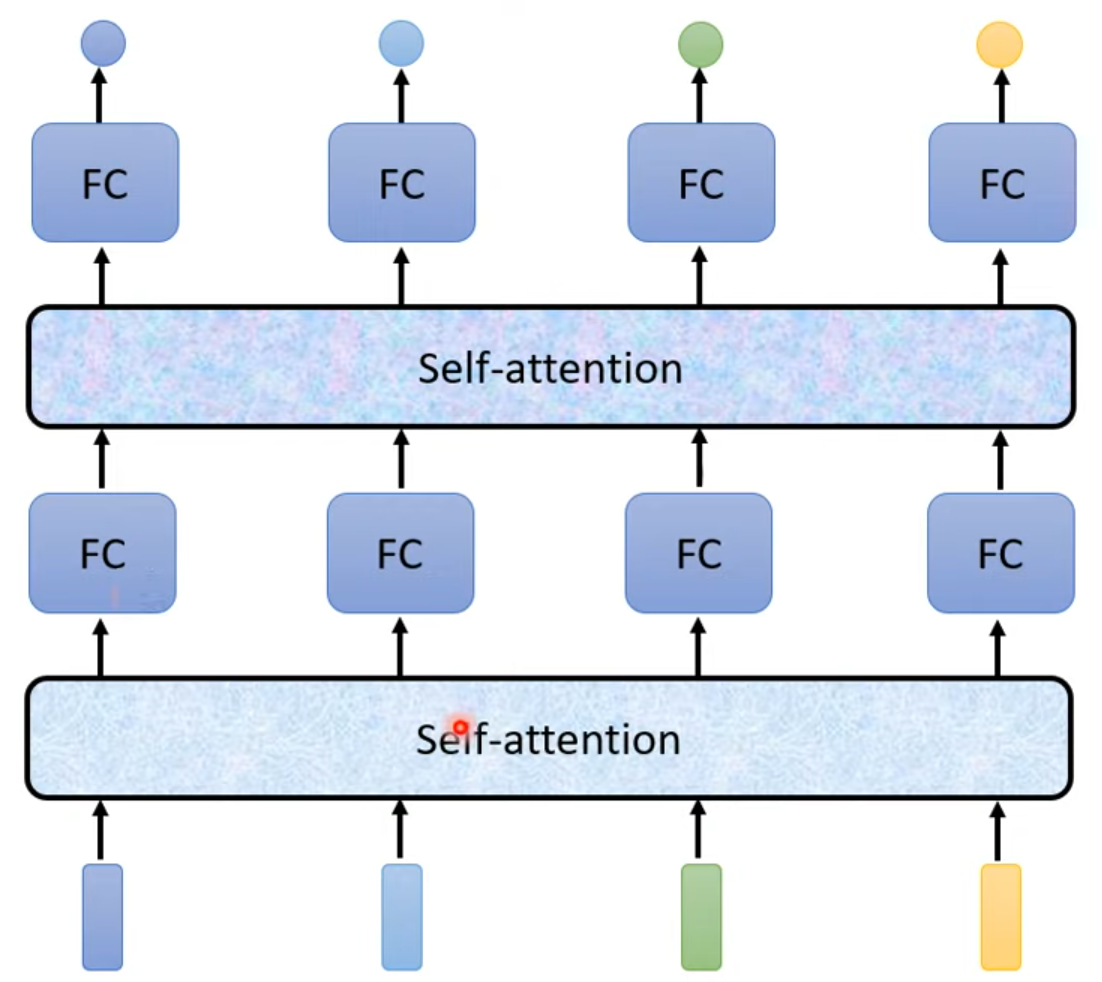
  • FC = fully-connected
  • use fully-connected to focus, use self-attention to consider the whole
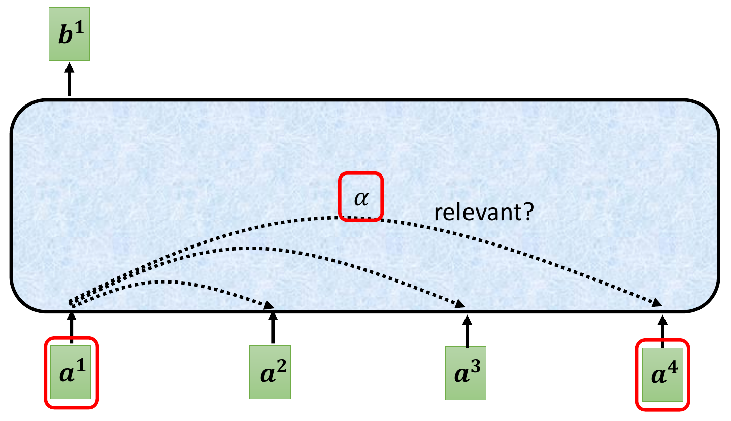
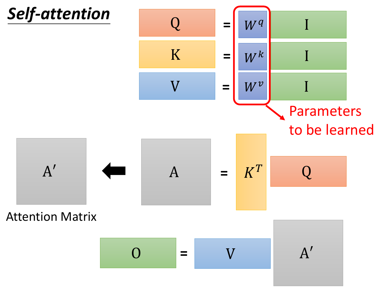
• computation
  • 
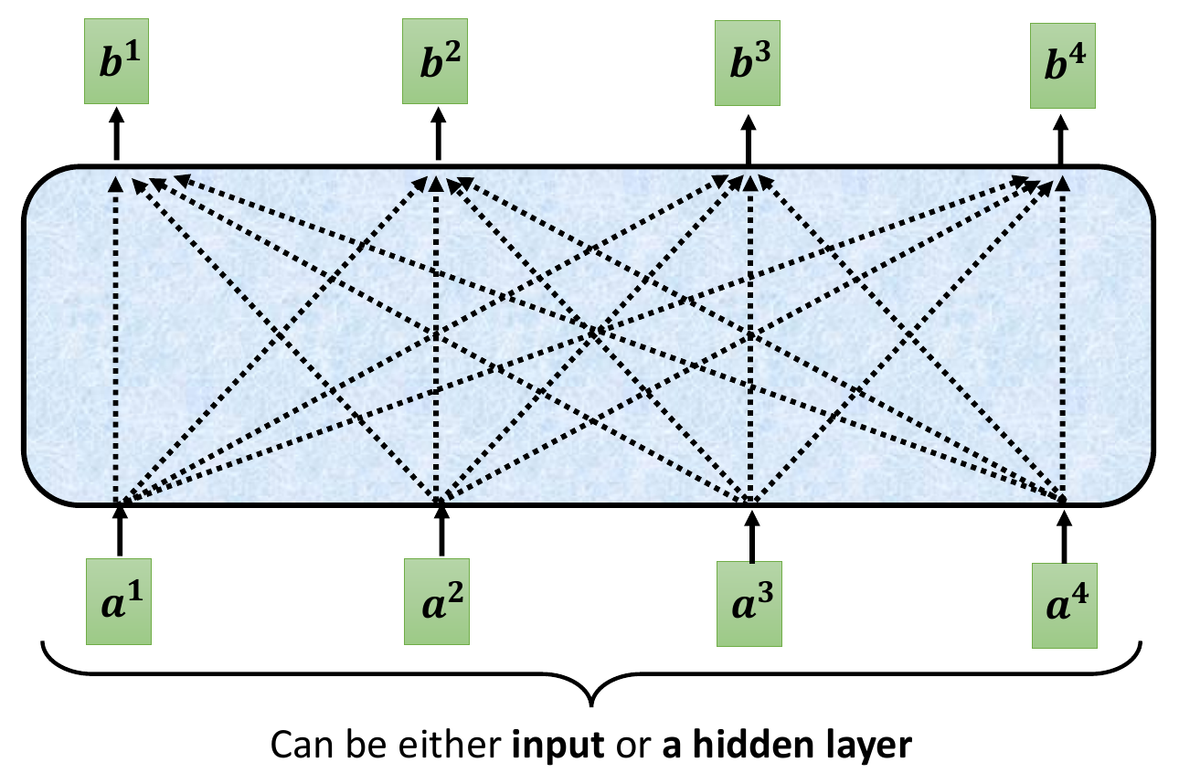
  • \(\alpha\) = attention score
    • the correlation between 2 vectors
      • 
    • 2 methods to compute
      • 
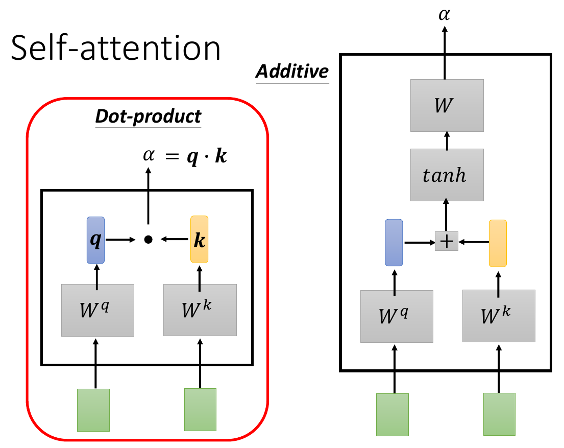
      • left is more common
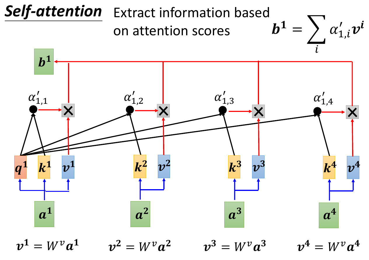
• get all \(\alpha\) and calculated weighted sum -> b1
  • 
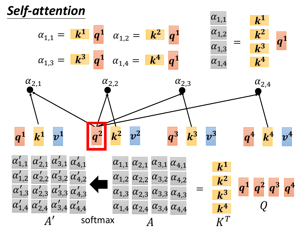
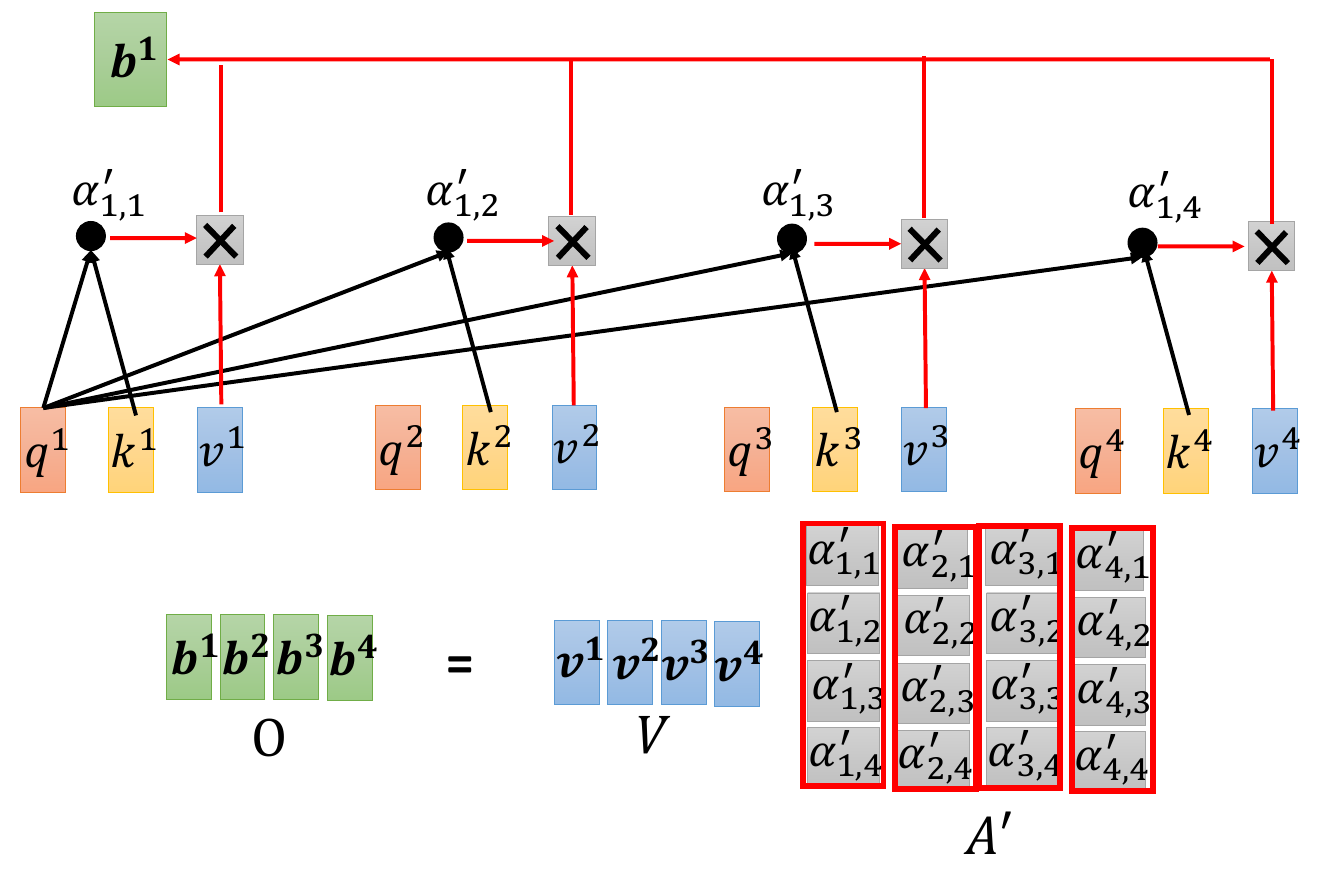
• full calculation
  • 
  • 
  • 
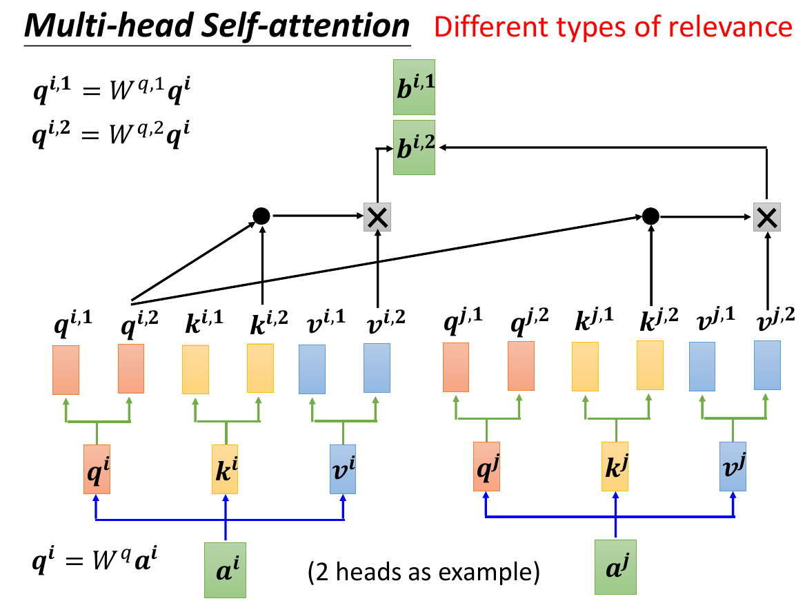
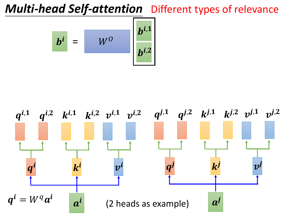
• multi-head
  • 
  • 
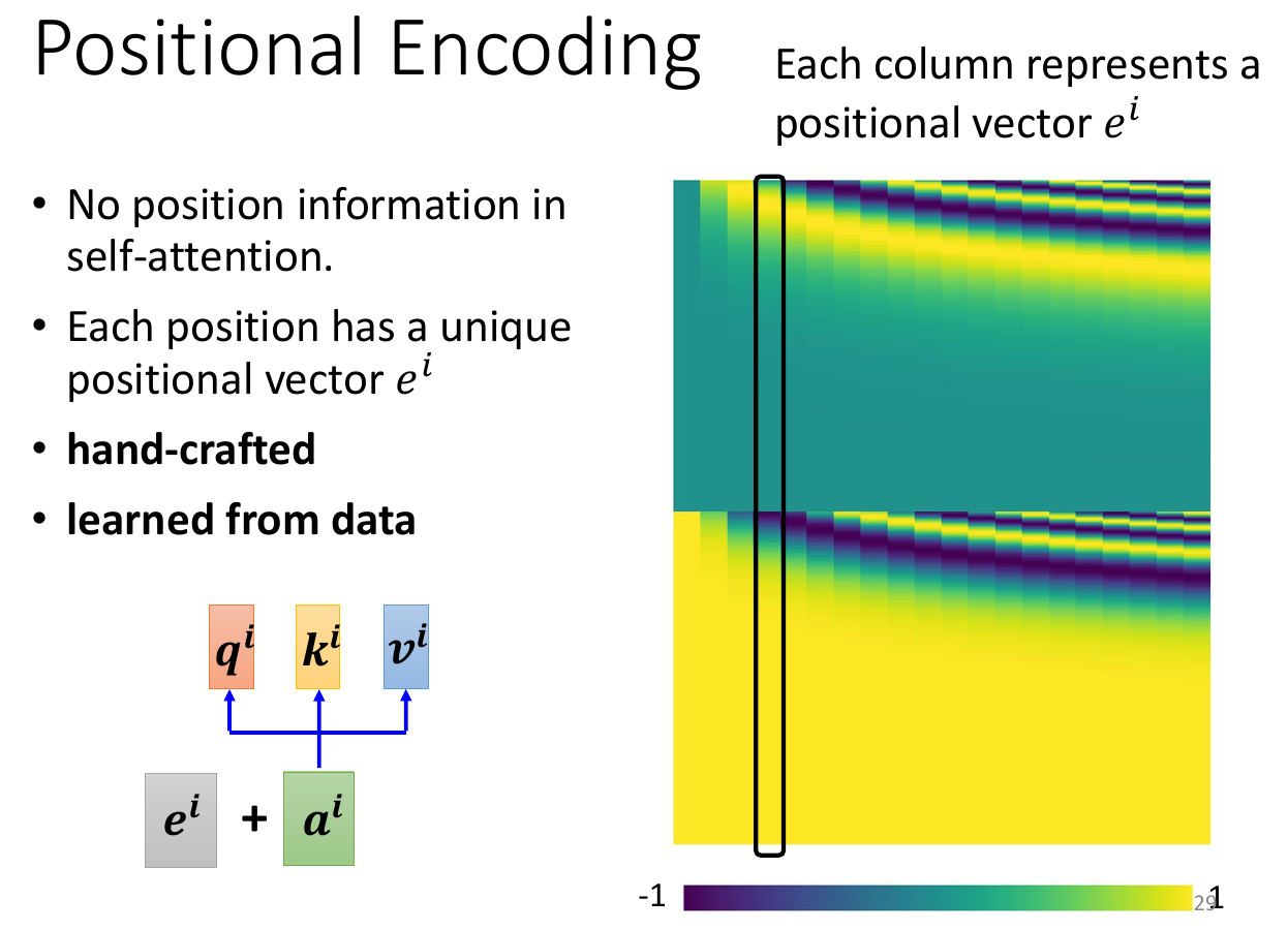
• positional
  • normal self-attention is indifferent to position -> add positional vector yourselfof
  • 
• truncated self-attention
  • not seeing the whole
  • speech
• CNN is a special case of self-attention
  • CNN is simplified self-attention (only see receptive field)
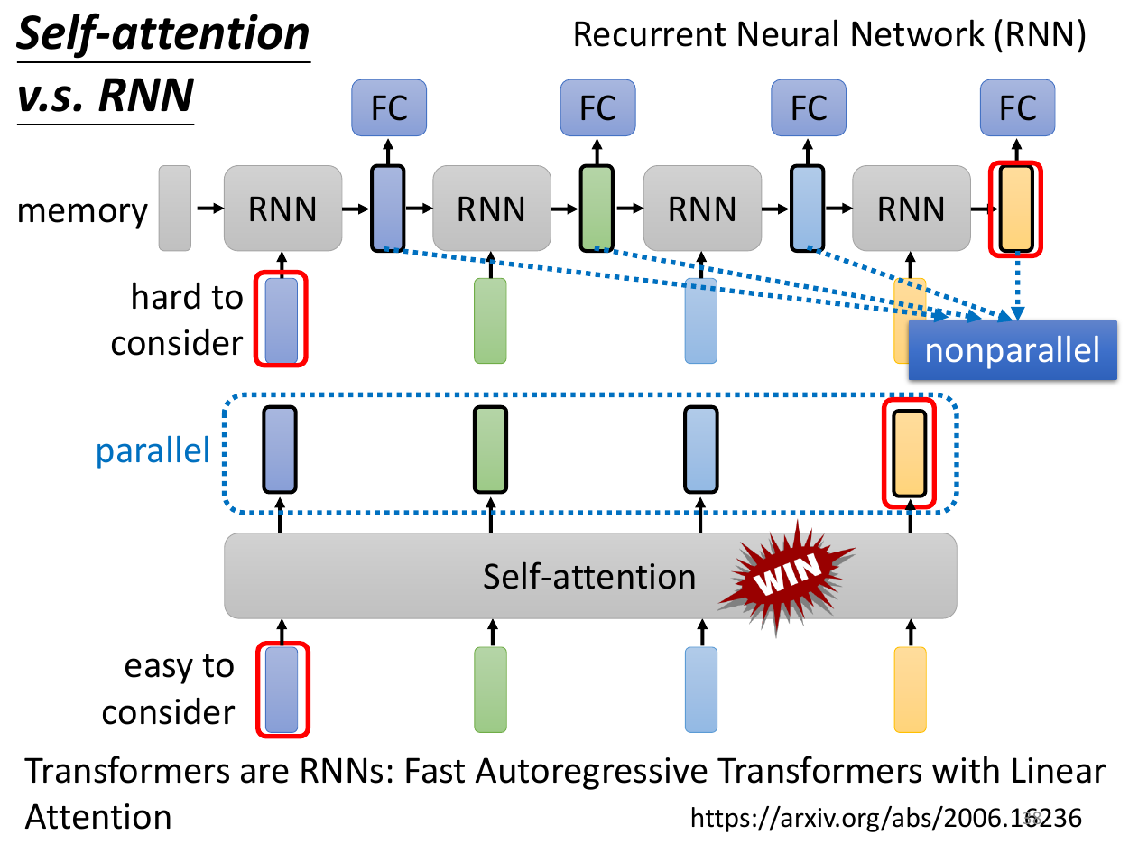
• RNN
  • recurrent neural network
  • largely replaced by self-attention
  • RNN is sequential -> slow
  • 

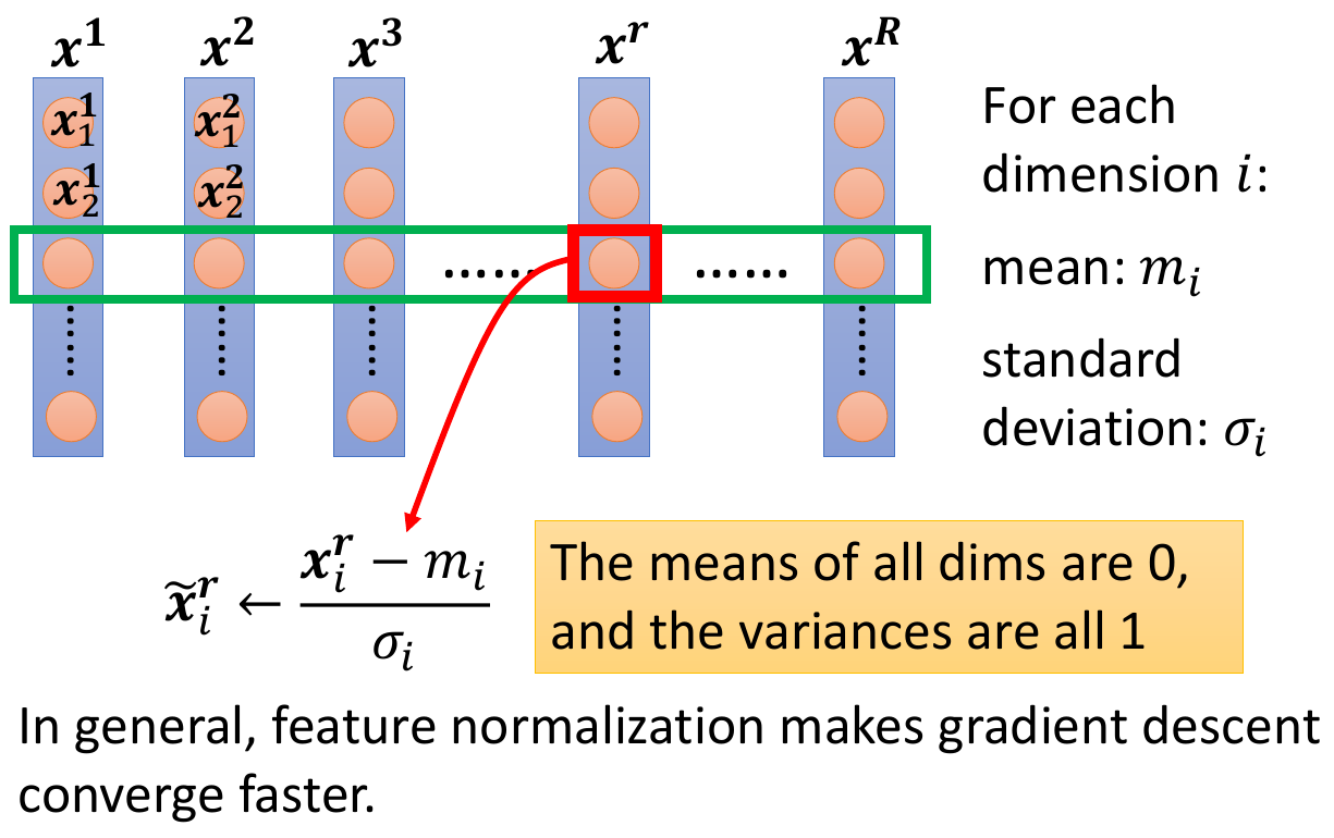
batch normalization

• feature normalization
  • normalize to mean = 0, variance = 1
    • 
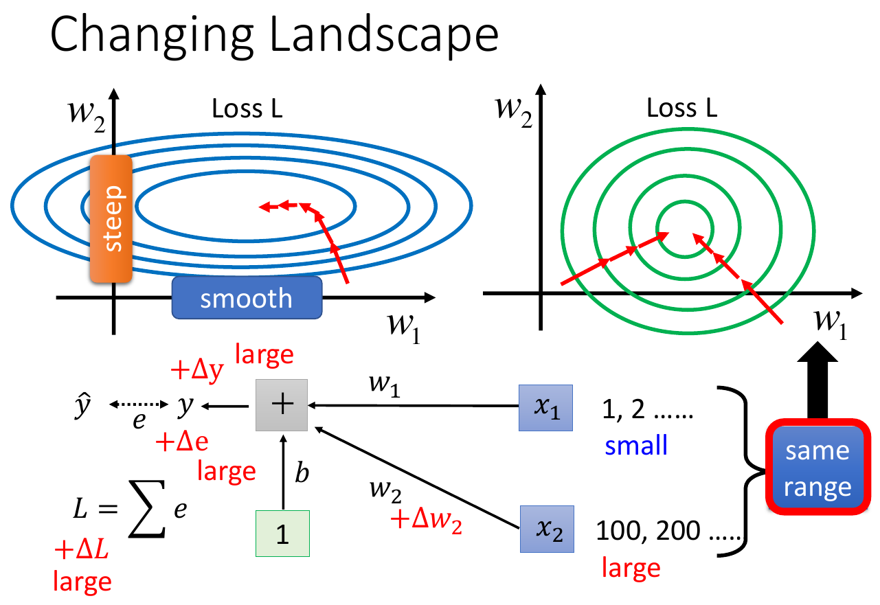
  • gradient descent converges faster after normalization
  • error surface changed
    • 
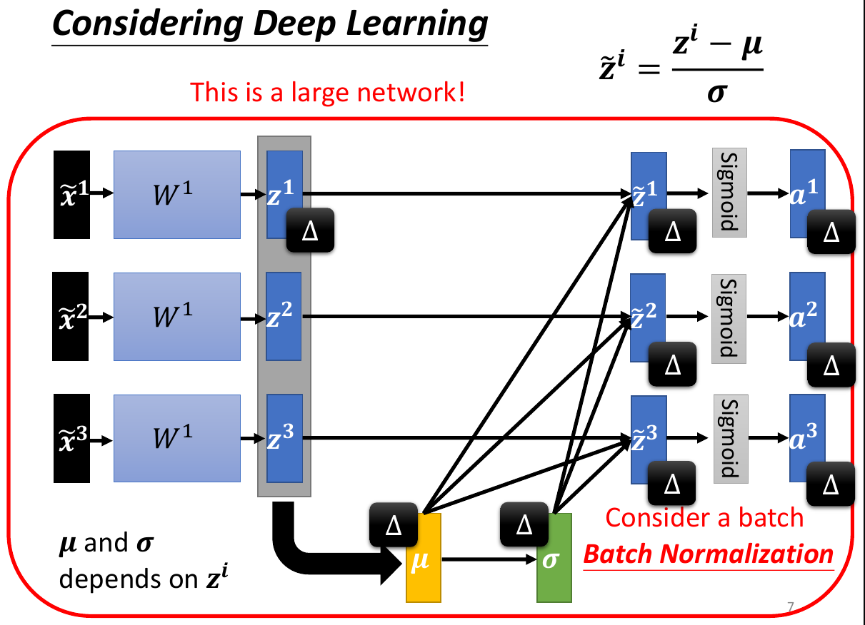
• batch normalization
  • 只對一個 batch 做 feature normalization
    • 
  • at testing, mean and std are calculated on a moving average basis
    • otherwise will need to wait for enought data to be able to calculate
    • 
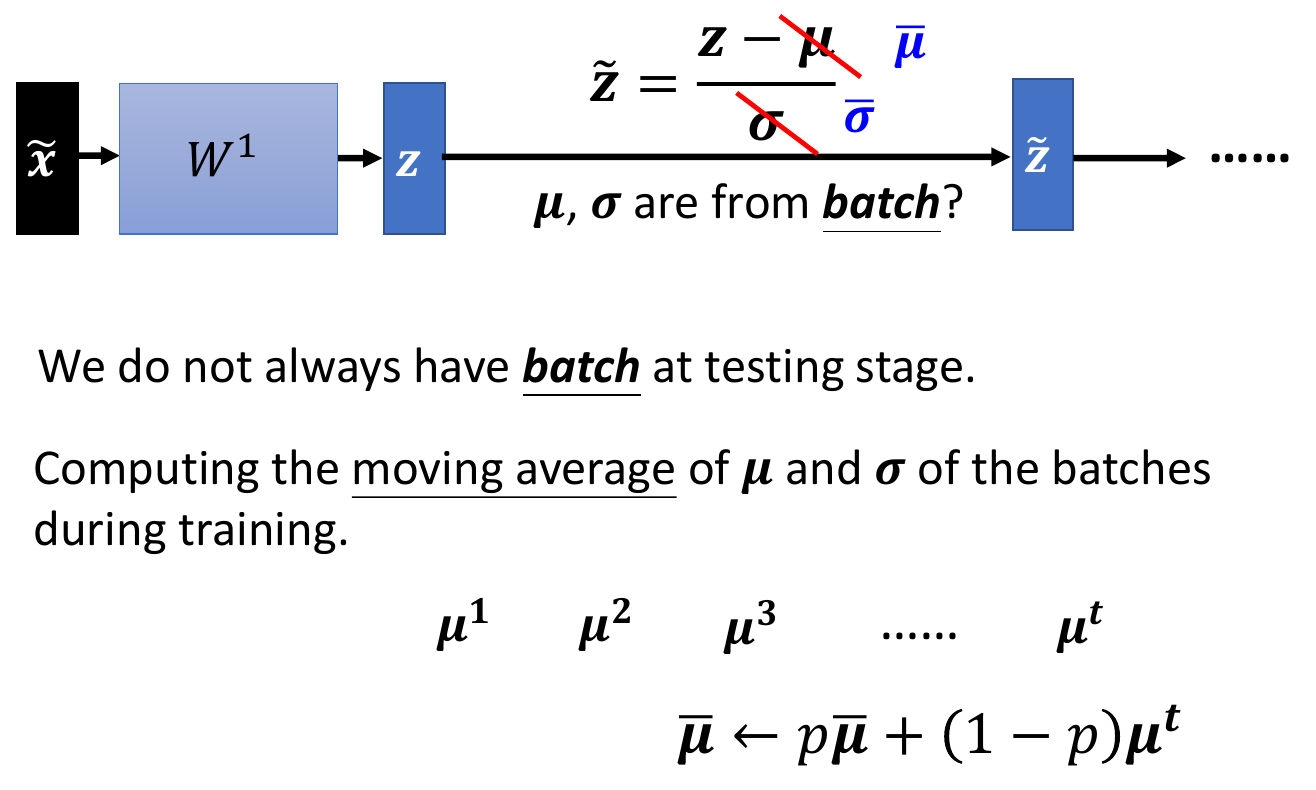
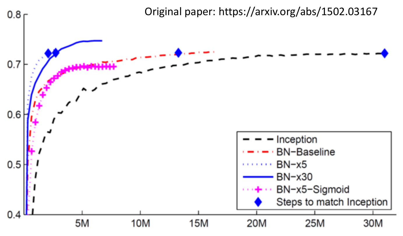
  • faster to converge (to the same accuracy)
    • 
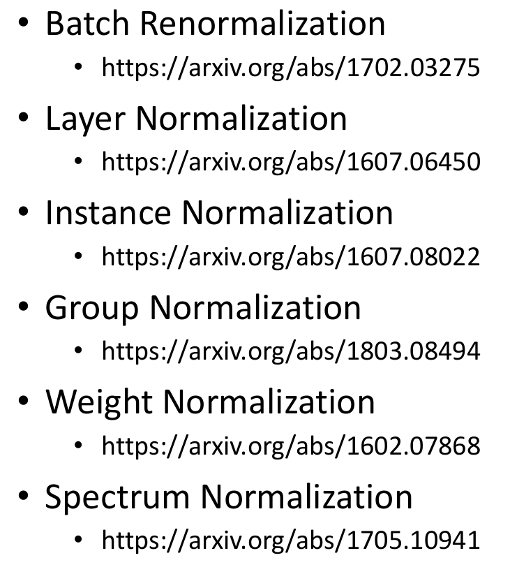
• batch normalization is one of the many normalization methods
  • 

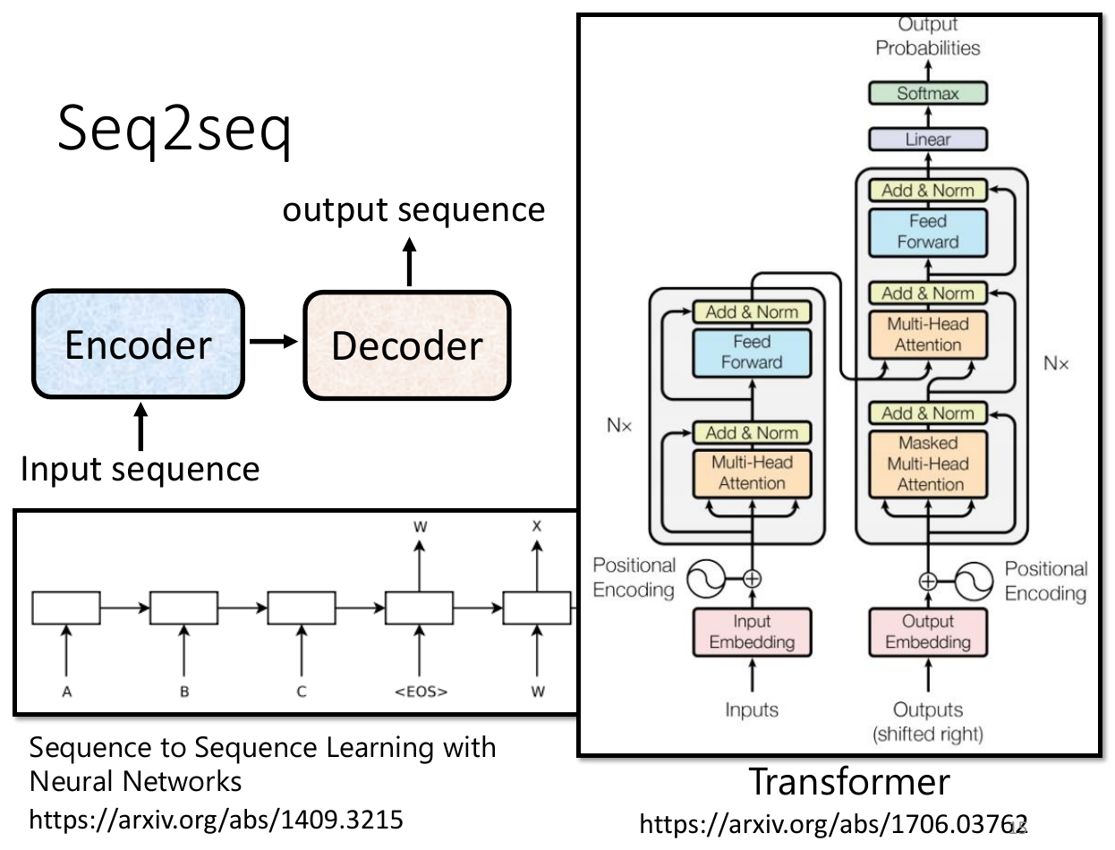
transformer

• seq2seq
  • input sequence, output sequence
  • decide size of output sequence itself
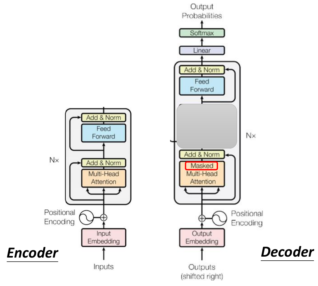
  • architecture
    • 
    • 
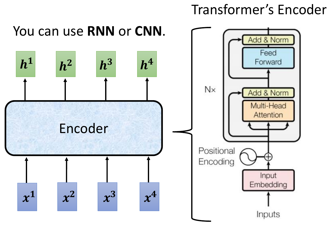
  • encoder
    • 
  • decoder
    • minimize cross entropy
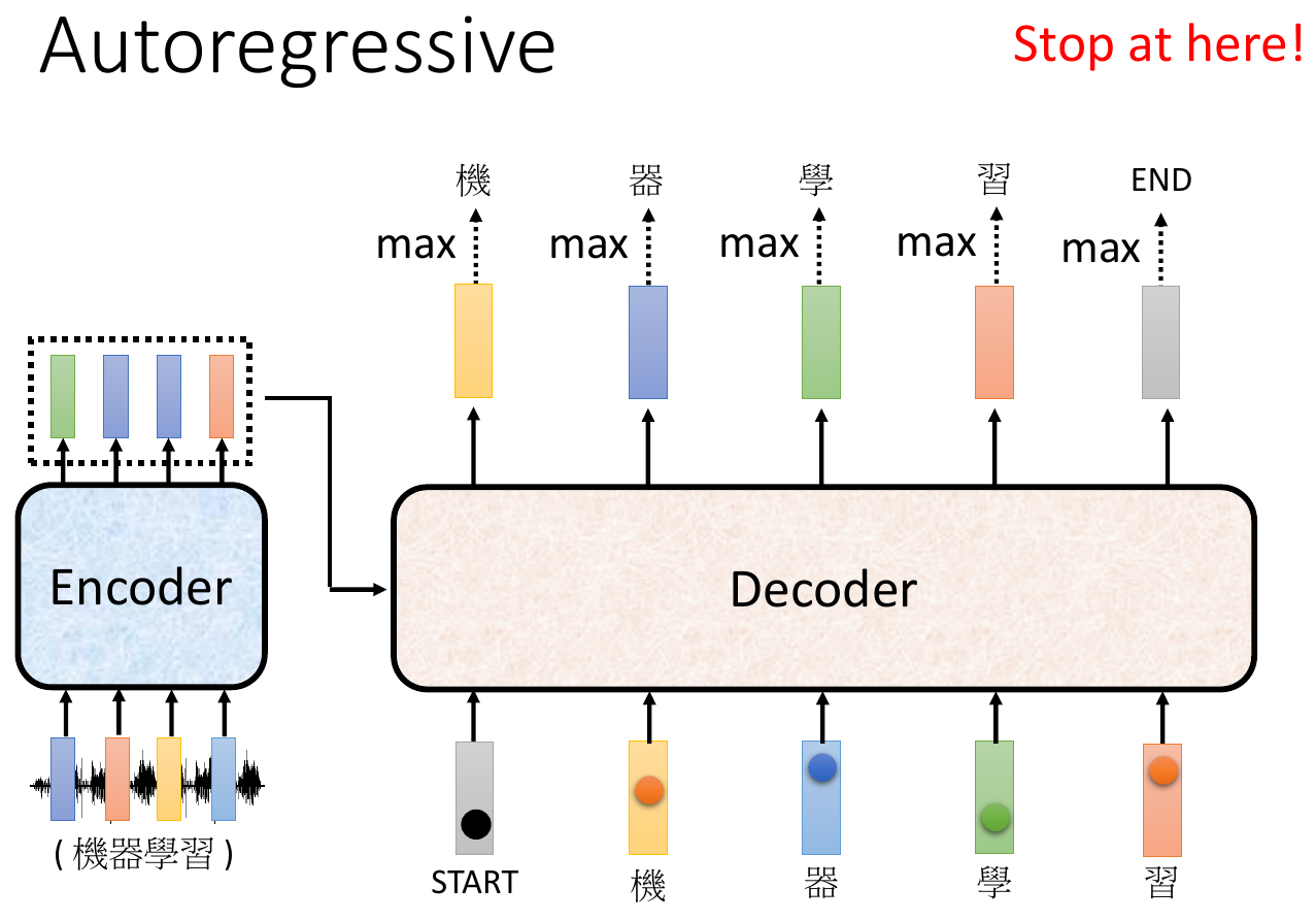
    • teacher forcing
      • give decoder correct value to teach it
    • a "Begin of Sentence" one-hot vector
    • output a stop one-hot vector -> terminate
      • 
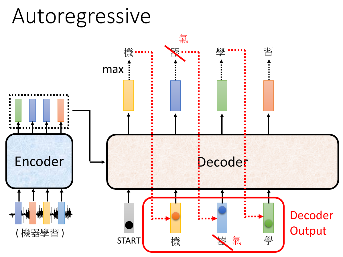
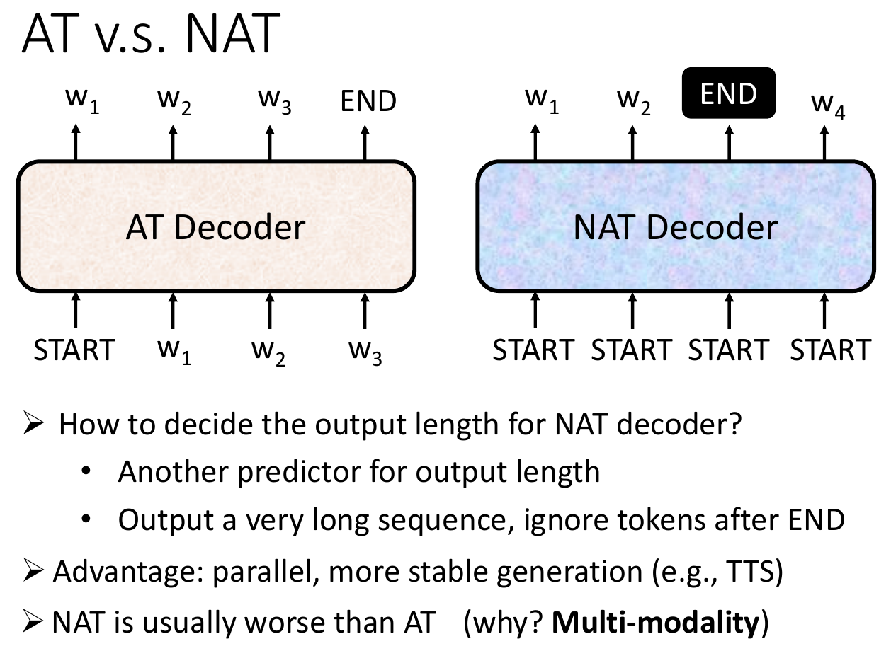
    • AT, autoregressive
      • take previous output as input (like RNN)
      • error may propagates
      • 
    • NAT, non-autoregressive
      • parallel
      • decoder performance worse than AT
      • 
• seq2seq usage
  • multi-label classification
    • decide hoe many class itself
  • object detection
• copy mechanism
  • pointer network
  • able to copy a sequence from input and output
  • 
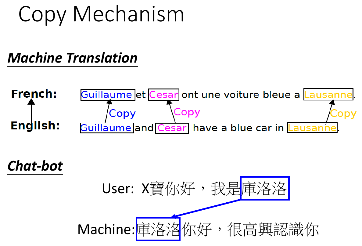
• summarization
• guided attention
  • force training in certain way
    • e.g. force left to right

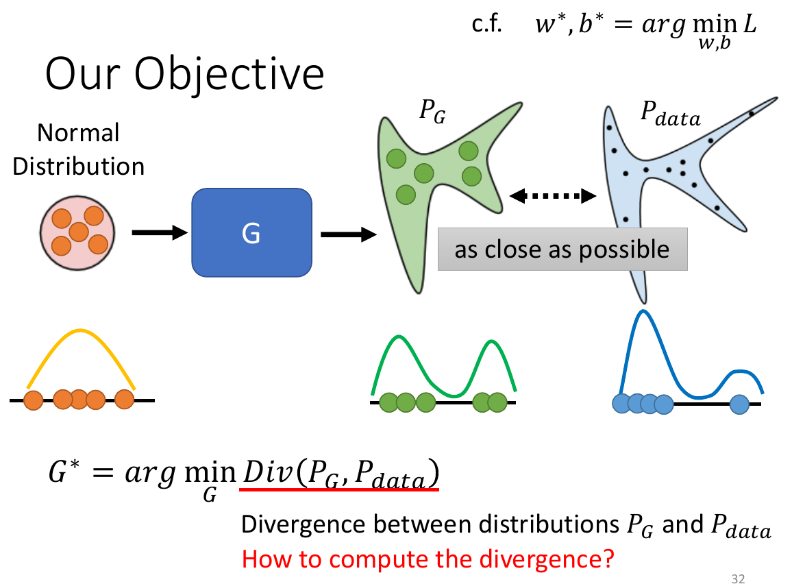
GAN

• generator adversarial network
• generator
  • input a vector, output an image
  • maximize the score of discriminator
• discriminator
  • a neural network output a scalar, indicating the realness of the input
  • using classification
    • real images = 1
    • generated images = 0
  • using regression
    • real images -> output 1
    • generated images -> output 0
• generator generates image, while discriminator finds out the difference between the real images and and ones from generator
  • both learn improve in the process
• algorithm
  • 交替 train
    • fix generator, train discriminator
    • fix discriminator, train generator
      • concat generator & discriminator but only update the parameters of generator
      • 
• theory
  • minimize the divergence
    • 
  • difficult to train
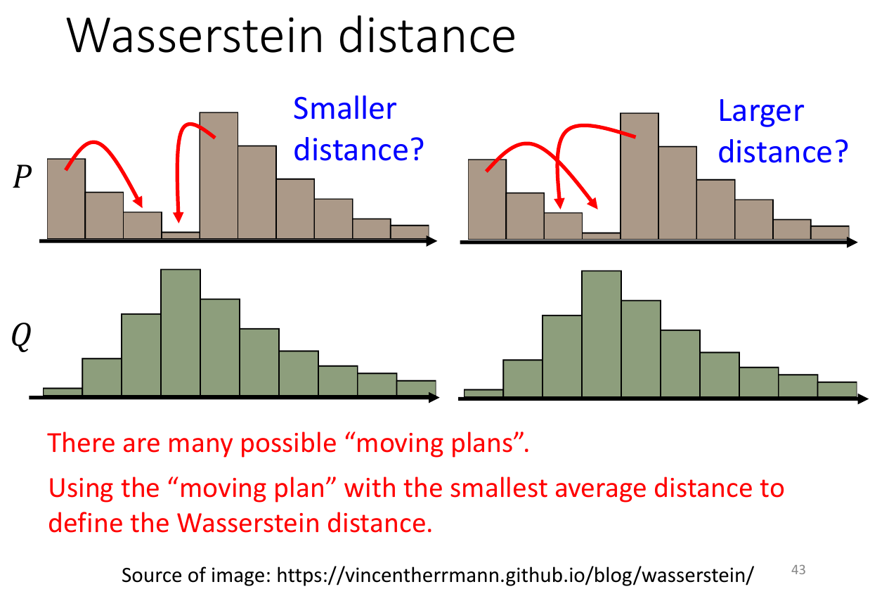
  • Wasserstein distance
    • min overhead needed to transform a distribution to another
    • 

Auto-Encoder

• autoencoder & variational autoencoder
  • https://towardsdatascience.com/ed7be1c038f2
  • https://towardsdatascience.com/f70510919f73
• self-supervised
  • no need label
• 
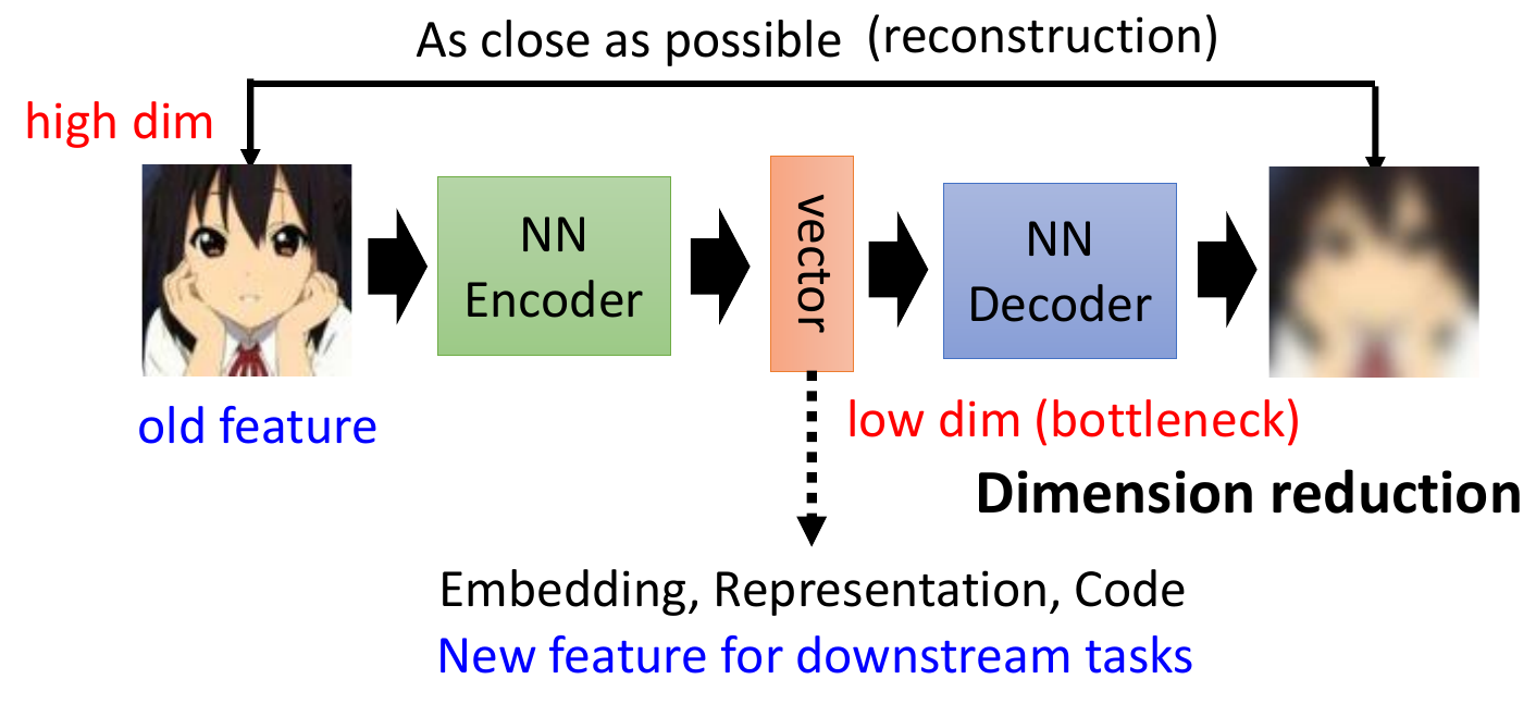
• encode high dim thing into low dim -> bottleneck
• decide low dim back to high dim

Explainable AI

Lime

• show the part of the image the model used to classify
• green -> positive correlation red -> negative correlation
• slice an image into many small parts, turn each on/off, and see the output change
  • like Econometrics
• references
  • https://www.oreilly.com/content/introduction-to-local-interpretable-model-agnostic-explanations-lime/
  • https://towardsdatascience.com/interpreting-image-classification-model-with-lime-1e7064a2f2e5

Saliency Map

• heatmap of the importance of pixels to the classficiation result
• visualization of the partial differential values of loss to input tensor
• reference
  • https://medium.datadriveninvestor.com/visualizing-neural-networks-using-saliency-maps-in-pytorch-289d8e244ab4

Smooth Grade

• add random noisy and generate saliency map

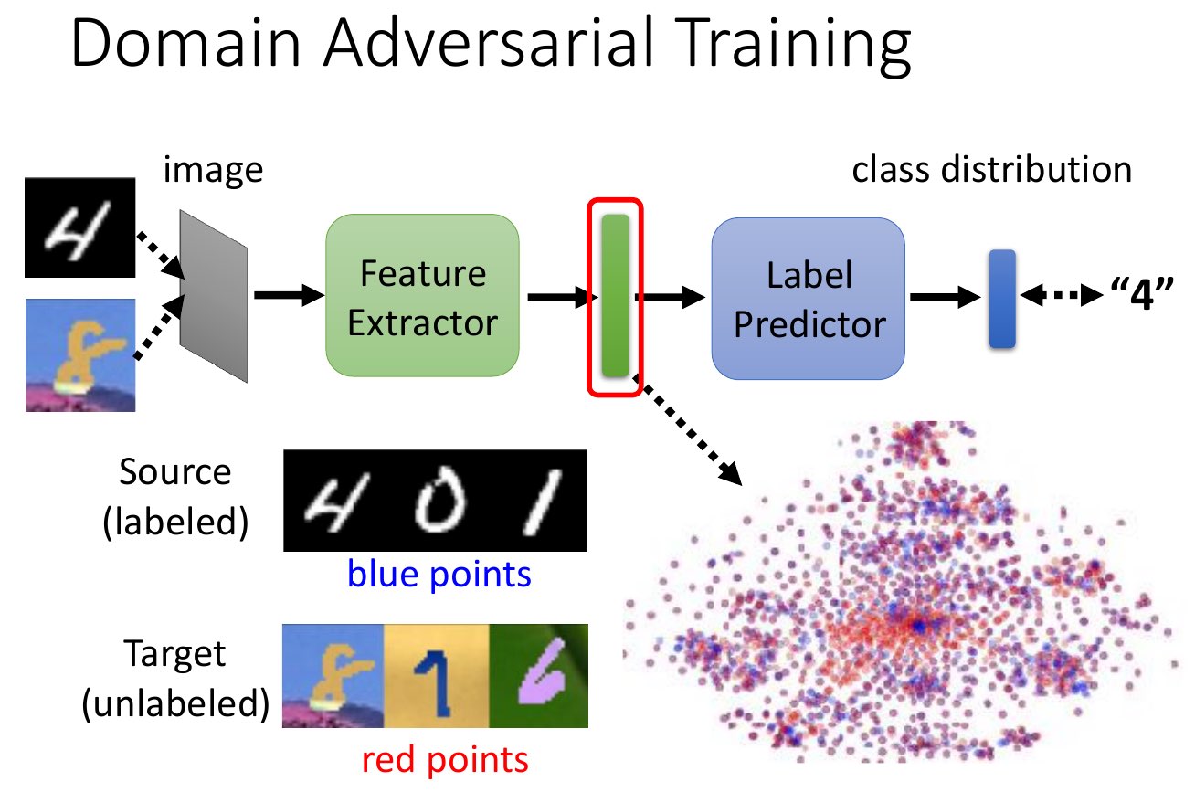
Domain Adaptation

• adapt a model into a different domain
  • e.g. similar but different form of data
  • 
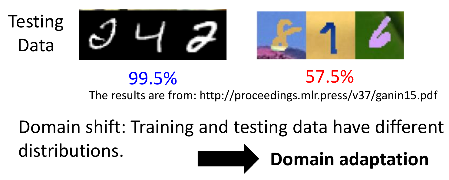
• use feature extractor to extract the key features
  • goal: feature extracted from source == from data
• use label predictor to predict the class from the extracted features
• 

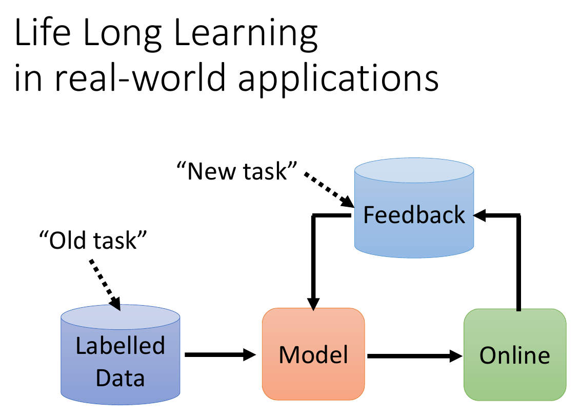
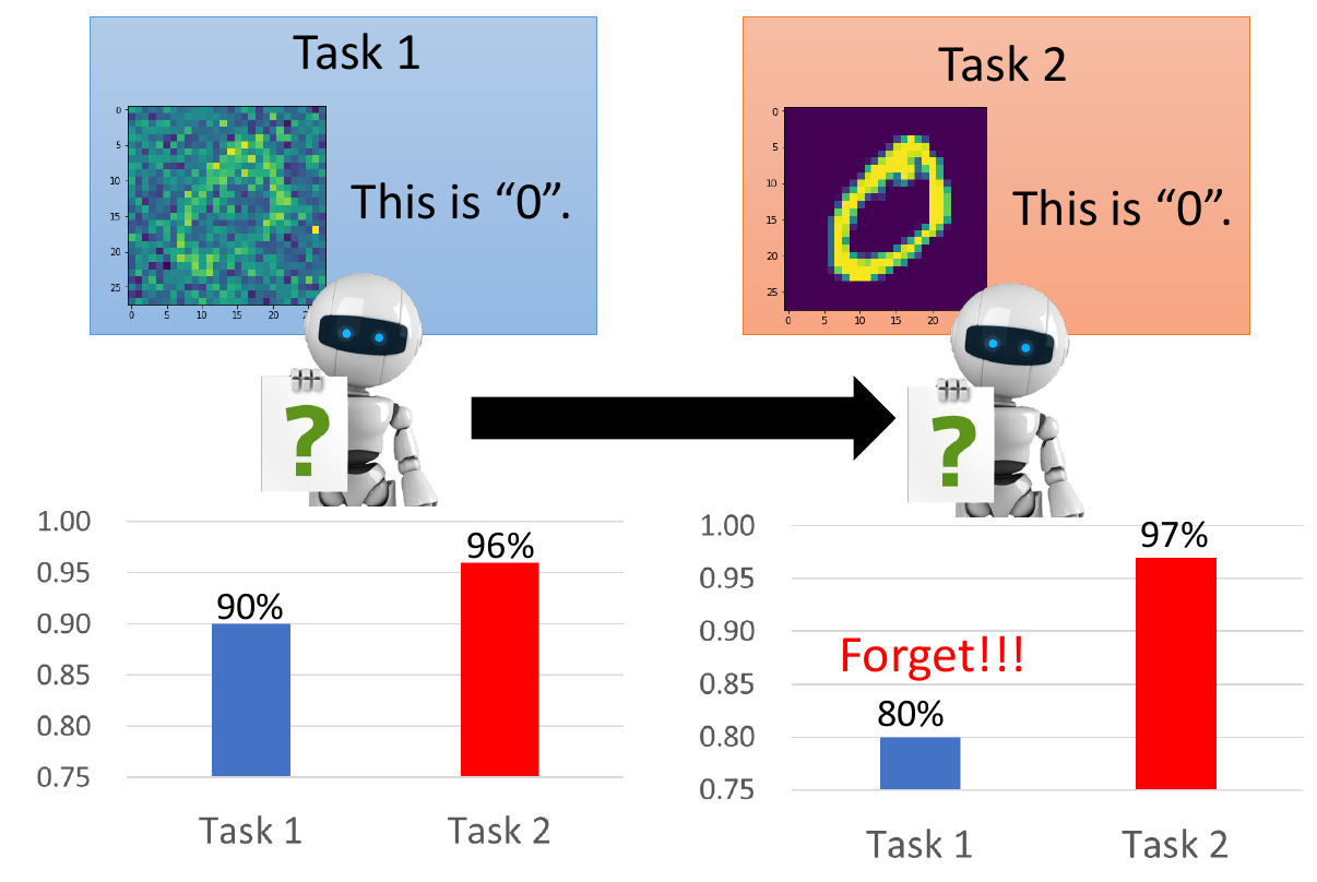
Life Long Learning

• learn new tasks continuonsly
  • can be new sets of data, new domains, etc.
  • 
• can't learn multiple tasks sequentially - catastrophic forgetting
  • 
• but can learn multiple tasks simultaneously - multi-task learning
  • 
  • 
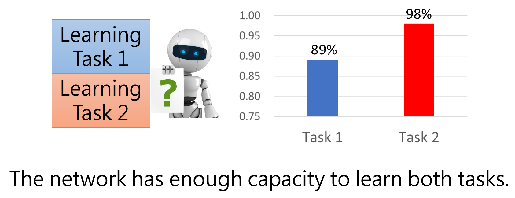
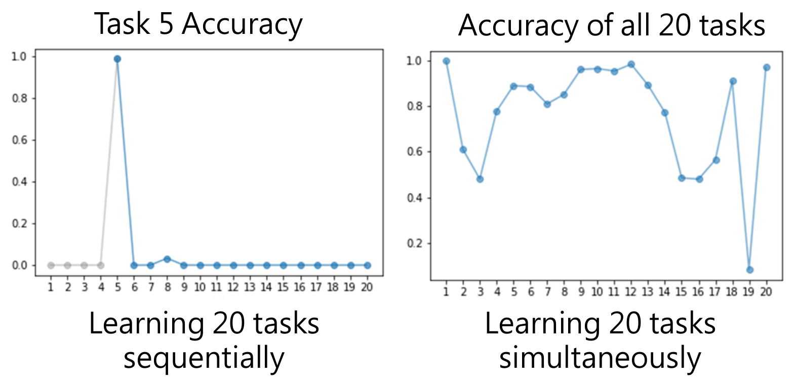
  • not practical
    • need to store all the task data
    • need extreme computation
  • upper bound of life long learning

Q Learning

• components
  • state
  • action
  • reward
• maximize future cummulative expected payoff

Bellman equation

• \(\alpha\) = learning rate
• \(\gamma\) = discount rate

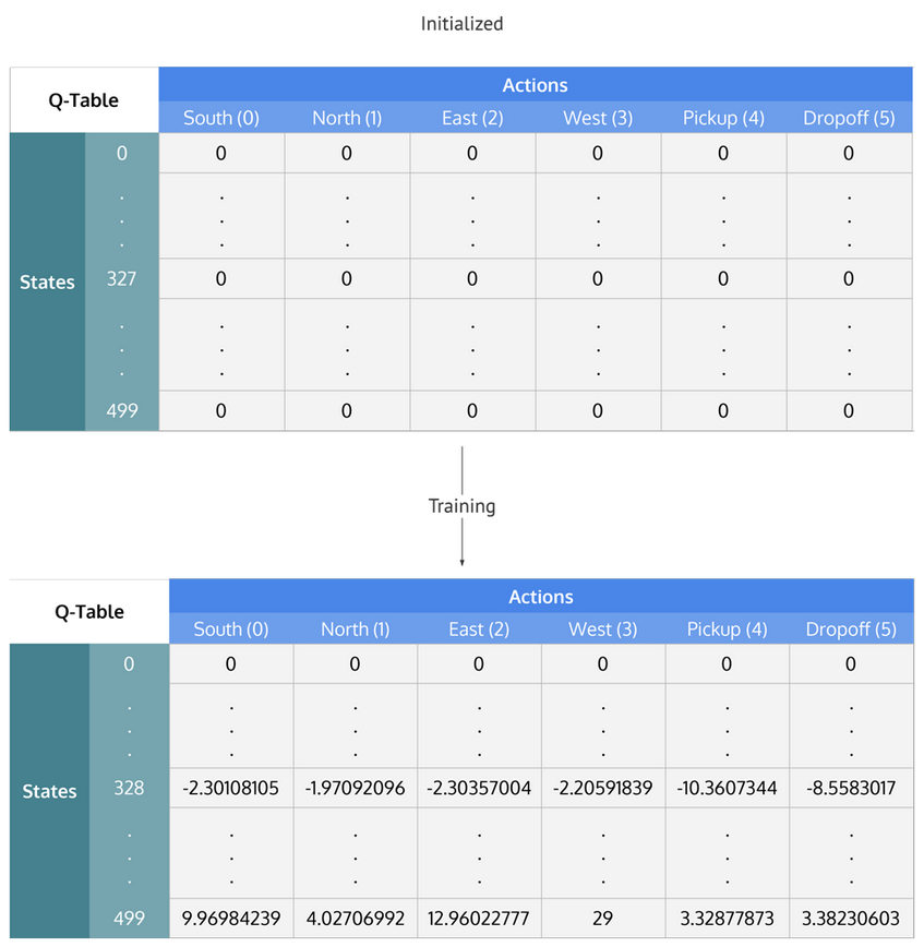
Q Table

If represent each state & each action as an interger

• row & column = state & action
• cell value = q value = discounted future total rewards
• iterate and update cell values (like dp)
  • given a state -> choose the action resulting to greatest q value -> update cell value & go to new state

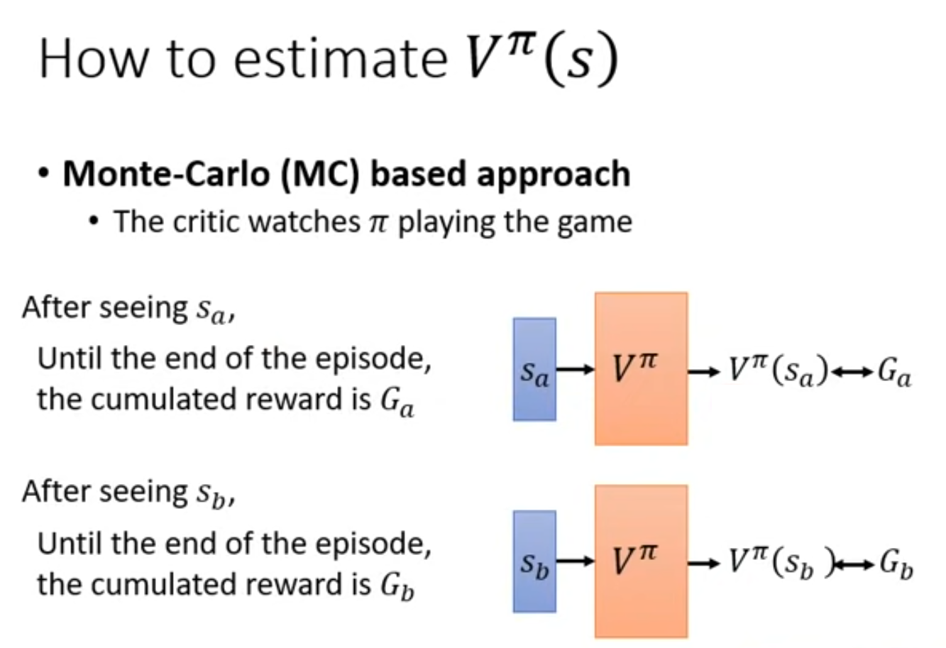
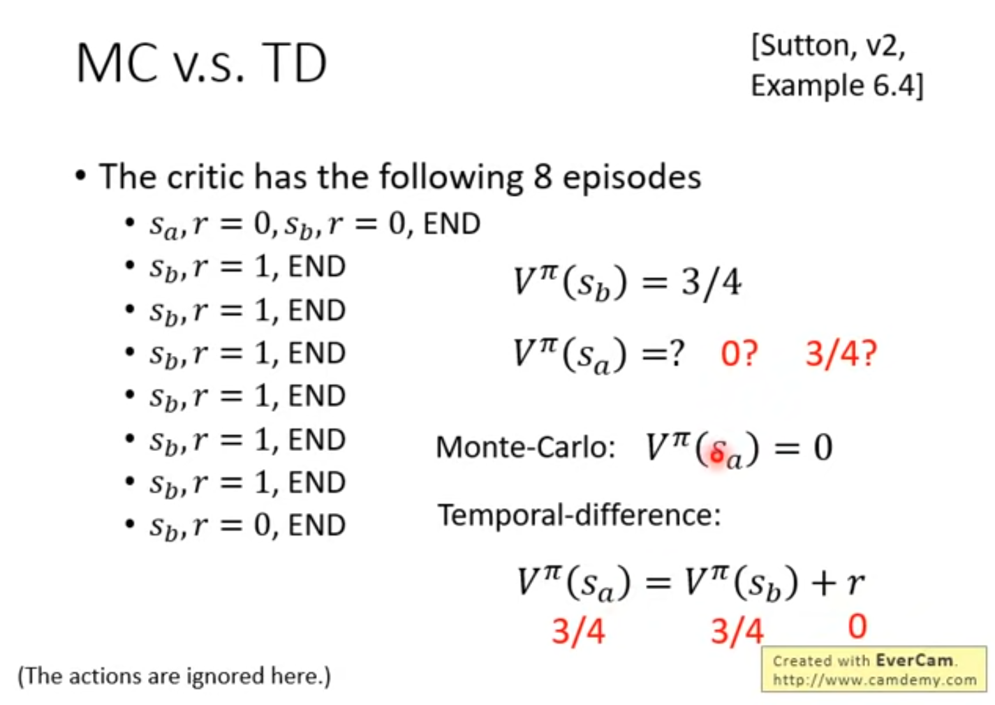
Monte-Carlo (MC)

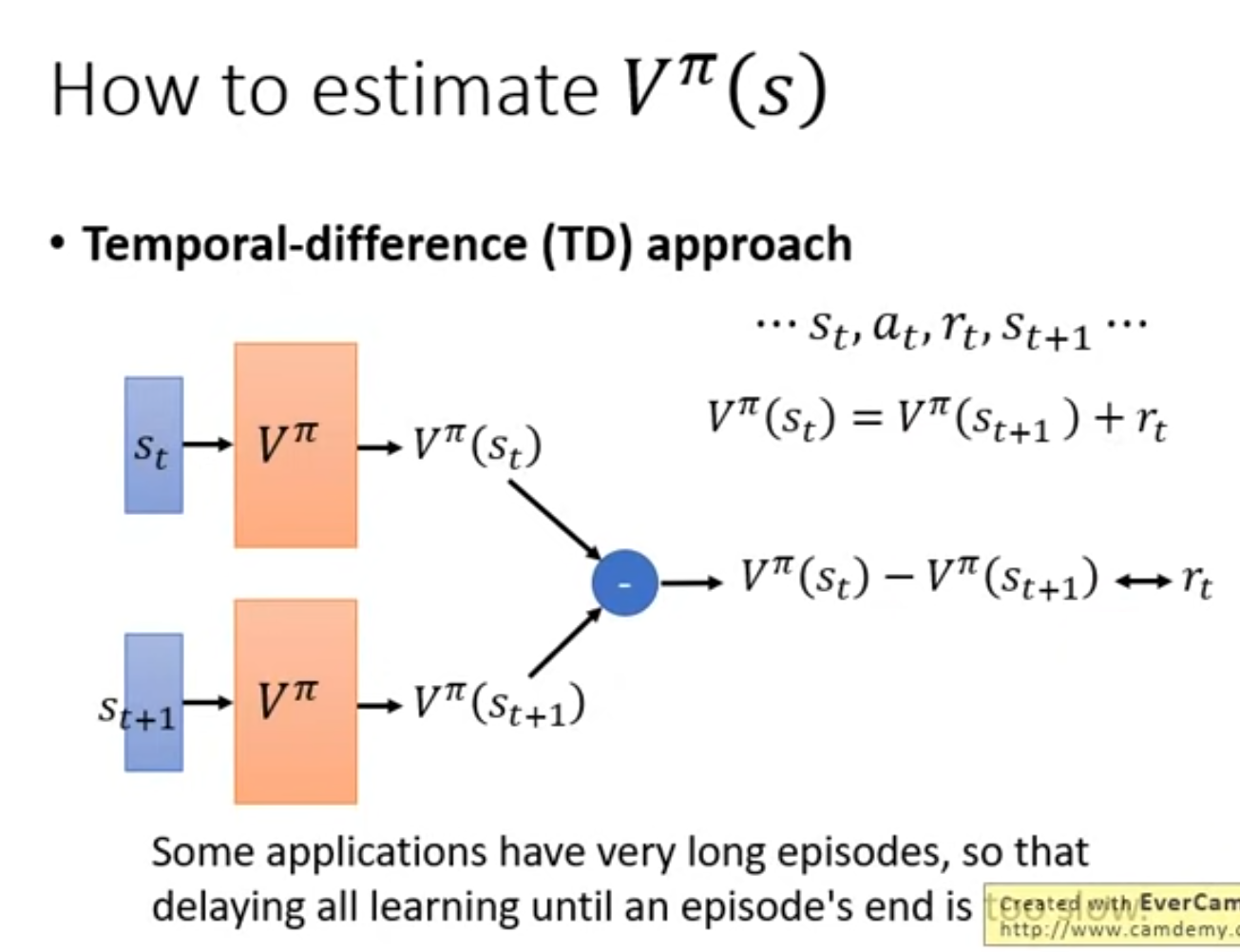
Temporal-difference (TD)

\(V^{\pi}(s_{t+1})\) = 下個 action 之後的 cummulative expected payoff = 現在 action 之後的 cummulative expected payoff - 這次的 reward

MC vs. TD

Deep Q Learning

https://towardsdatascience.com/2a4c855abffc

Q Learning but replace Q table with neural network

• input: state
• output: action -> reward

Still need to update Q value with Bellman equation