International Finance

Ch1 Balance of Payment

國際收支表

• 金融帳 FA (financial account)
  • \(\Delta\) 金融性資產
  • 國外金融資產淨額 NFA (net foreign asset) \(B_t=a^f_t-a^h_t\)
    • \(a^f\) = 本國居民持有國外金融資產
    • \(a^h\) = 外國居民持有本國金融資產
  • \(FA_t=-(B_{t+1}-B_t)\)
  • NFA 增加 -> 逆超
• 官方準備帳 ORA (official reserve account)
  • \(\Delta\) 國外資產/外匯存底 foreign exchange reserves
  • \(ORA=-(H_{t+1}-H_t)\)
  • \(H\) = 央行持有國外資產
• 經常帳 CA (current account)
  • sum of
    • imports and exports of goods and services \(X_t-M_t\)
    • investment income \(X_{FS,t}-M_{FS,t}\)
    • unilateral transfers \(UT_{IN,t}-UT_{OUT,t}\)
      • directly giving/receiving money to/from foreign citizens
  • \(CA_t=TB_t+NFI_t\)
  • 貿易帳 trade account \(TB_t=X_t-M_t\)
  • 國外所得淨額 \(NFI_t=(X_{FS,t}-M_{FS,t})+(UT_{IN,t}-UT_{OUT,t})\)
• 資本帳 KA (capital account)

\[CA+FA+KA+ORA=0\]

Assuming \(KA=0\), if \(CA>0\)

• 央行不干預 \(\rightarrow ORA=0 \rightarrow FA=-CA<0\)
• 央行小干預 \(\rightarrow 0<-ORA<CA \rightarrow FA=-CA-ORA<0\)
• 央行大干預 \(\rightarrow 0<CA<-ORA \rightarrow FA=-CA-ORA>0\)

When \(KA=0\)

• \(CA+FA+ORA=0\)
• \(CA=-FA-ORA=(B_{t+1}-B_t)+(H_{t+1}-H_t)\)
  • 民間國外資產變動 + 官方國外資產變動

Formulas

\[GNI=GDP+NFI\]

\[GDP=Y=C+I+G+(X-M)\]

\[CA=(X-M)+NFI\]

See Macroeconomics#支出面 & Macroeconomics#國民儲蓄 national saving

• NFI = net foreign income
• CA = current account
• fiscal deficit is when \(T-G<0\)

\[\begin{align*} & GNI\\ &= C+I+G+CA\\ &= C+I+T+(G-T)+CA \end{align*}\]

\[CA=(GNI-C-I-T)+(T-G)\]

So a bigger fiscal deficit leads to smaller current account

Problems

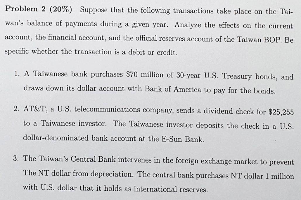
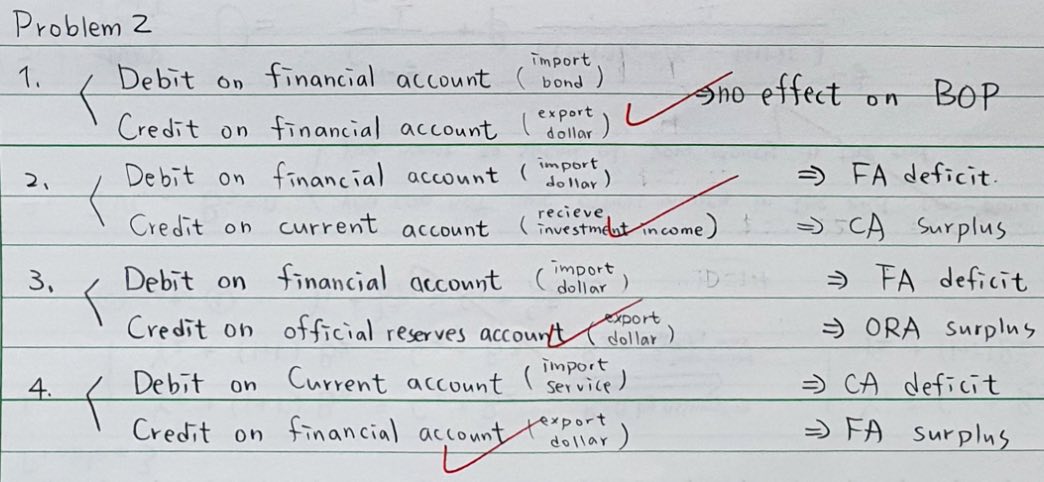
Ch2 Intertemporal Models of Current Account Dynamics

two-period endowment model

See also Macroeconomics#費雪兩期模型

Notations

• \(Y\) = endowment
• \(C\) = consumption
• \(r\) = interest rate
• \(\beta\) = time preference factor

Equilibrium

Problem formulation

\[\begin{align*} & \max_{\{C_1,C_2\}}u(C_1)+\beta u(C_2)\\ & s.t. Y_1+\dfrac{Y_2}{1+r}=C_1+\dfrac{C_2}{1+r} \end{align*}\]

First order condition

We know

\[C_2=Y_2+(1+r)(Y_1-C_1)\]

So

\[u'(C_1)-\beta u'(C_2)(1+r)=0\]

\[u'(C_1)=\beta u'(C_2)(1+r)\]

It's also called the Euler equation

current account

\[Y_t+(1+r)B_t=C_t+B_{t+1}\]

Assume there's no 央行 so

\[\begin{align*} & CA_t=(B_{t+1}-B_t)+(H_{t+1}-H_t)\\ &= B_{t+1}-B_t\\ &= Y_t+rB_t-C_t \end{align*}\]

In 2-period model \(B_1=B_3=0\)

\[CA_1=B_2-B_1=B_2=Y_1-C_1\]

\[CA_2=B_3-B_2=-B_2=Y_2+rB_2-C_2\]

\[CA_1=-CA_2\]

只有兩期 so 一二期 current account 順替差相抵

Assume \(u(C)=\ln C\)

We know

• \(u'(C_1)=\beta u'(C_2)(1+r)\)
• \(C_1+\dfrac{C_2}{1+r}=Y_1+\dfrac{Y_2}{1+r}\)

So

• \(C_2=\beta C_1(1+r)\)
• \((1+\beta)C_1=Y_1+\dfrac{Y_2}{1+r}\)
• \(C_1=\dfrac{1}{1+\beta}(Y_1+\dfrac{Y_2}{1+r})\)
  • \(C_1\) is a function of lifetime wealth -> fit Macroeconomics#恆常所得假說 permanent income
  • MPC (marginal propensity to consume) = \(\dfrac{dC_1}{dY_1}=\dfrac{1}{1+\beta}\)
• \(C_2=\dfrac{\beta}{1+\beta}(1+r)(Y_1+\dfrac{Y_2}{1+r})\)
• \(CA_1=Y_1-C_1=\dfrac{\beta}{1+\beta}Y_1-\dfrac{1}{(1+\beta)(1+r)}Y_2\)
  • \(\dfrac{dCA_1}{dY_1}=\dfrac{\beta}{1+\beta}>0\) meaning CA is pro-cyclical

Autarky

At \(r=r^A\) there's no incentive to borrow or lend

\[C_1=Y_1\]

\[C_2=Y_2\]

\[\begin{align*} & u'(C_1)=\beta u'(C_2)(1+r)\\ &= u'(Y_1)=\beta u'(Y_2)(1+r^A) \end{align*}\]

\(r\) & \(\rho\)

If \(r=\rho\)

• \(\beta=\dfrac{1}{1+\rho}=\dfrac{1}{1+r}\)
• \(u'(C_1)=\beta u'(C_2)(1+r)=u'(C_2)\)
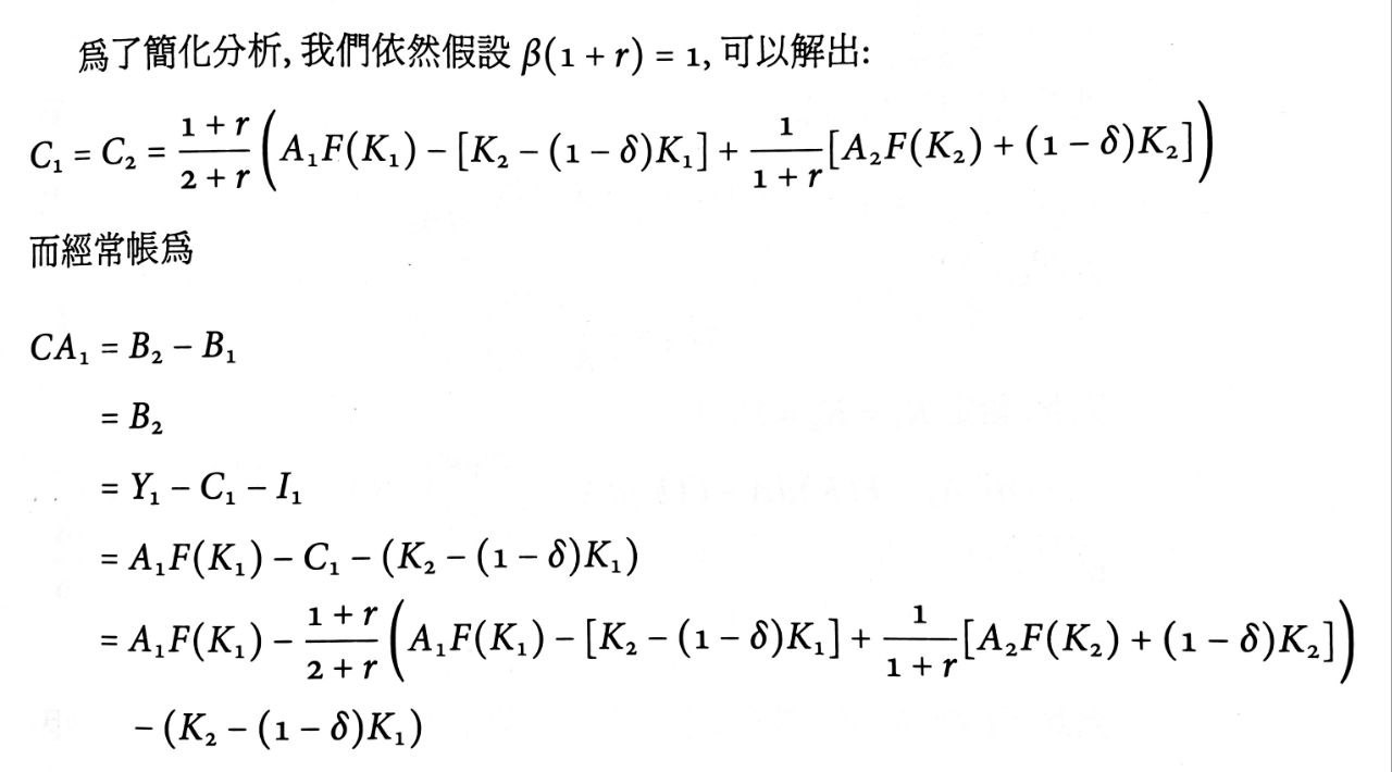
• \(C_1=C_2=\dfrac{1+r}{2+r}(Y_1+\dfrac{Y_2}{1+r})\)
• \(CA=Y_1-C_1=\dfrac{1}{2+r}(Y_1-Y_2)\)
  • \(Y_1>Y_2\) -> current account 順差
    • vice versa
  • if 所得恆常性增加 \(dY_1=dY_2\), then \(CA\) not changed
  • if 只有當其所得增加 \(dY_1>0\) & \(dY_2=0\), then \(CA\) 增加
    • vice versa

If \(\rho>r\) and \(Y_1=Y_2=Y\)

• \(\beta=\dfrac{1}{1+\rho}<\dfrac{1}{1+r}\)
• \(u'(C_1)=\beta u'(C_2)(1+r)<u'(C_2)\)
• \(C_1>C_2\)
• \(C_1+\dfrac{C_1}{1+r}>C_2+\dfrac{C_2}{1+r}=Y+\dfrac{Y}{1+r}\)
• \(C_1>Y\)
• \(CA_1=Y-C_1<0\)

Vice versa, if \(\rho<r\) and \(Y_1=Y_2=Y\), \(CA_1>0\)

two-period endowment model with government purchases

\[G_t=T_t\]

budget constraint

\[Y_t-T_t+(1+r)B_t=C_t+B_{t+1}\]

lifetime wealth

\[Y_1-T_1+\dfrac{1}{1+r}(Y_2-T_2)=C_1+\dfrac{C_2}{1+r}\]

\[Y_1-G_1+\dfrac{1}{1+r}(Y_2-G_2)=C_1+\dfrac{C_2}{1+r}\]

assume \(r=\rho\)

\[C_1=C_2=\dfrac{1+r}{2+r}(Y_1-G_1+\dfrac{1}{1+r}(Y_2-G_2))\]

\[\begin{align*} & CA_t=(B_{t+1}-B_t)+(H_{t+1}-H_t)\\ &= B_{t+1}-B_t\\ &= Y_t+rB_t-C_t-G_t \end{align*}\]

\[CA_1=Y_1-C_1-G_1=\dfrac{(Y_1-G_1)+(Y_2-G_2)}{2+r}\]

• 政府支出恆常性變動 \(dG_1=dG_2\) won't affect current account
• 政府支出短暫變動 \(dG_1>dG_2=0\) decreases current account

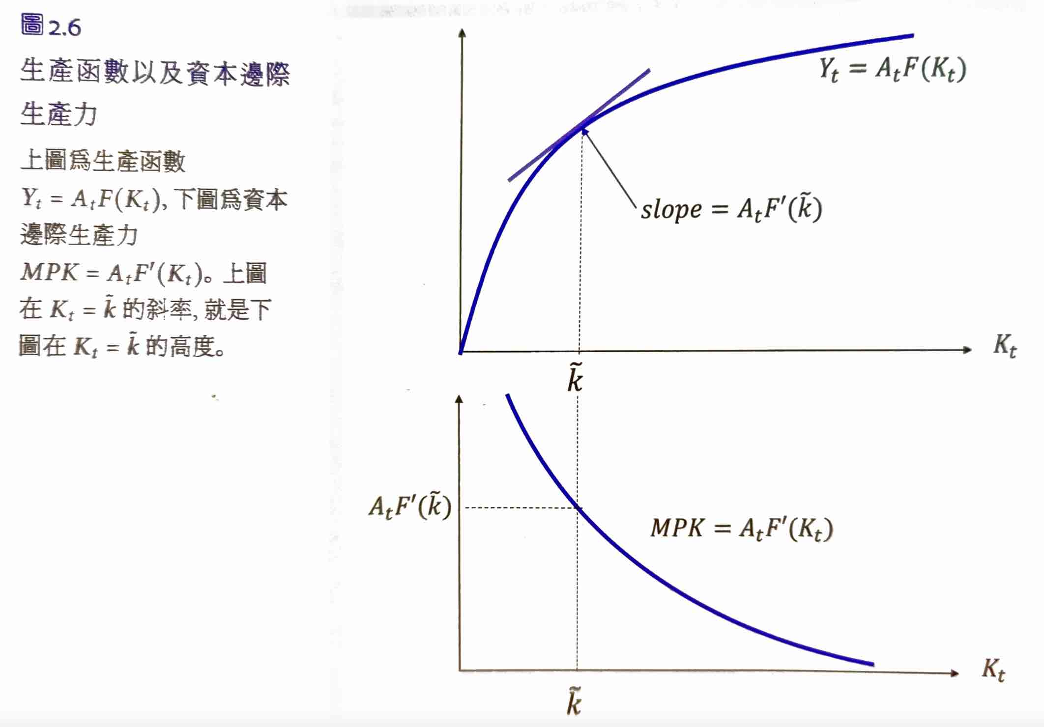
two-period model with production & investment

\[Y_t=A_tF(K_t)\]

• \(A_t\) = total factor productivity (TFP)
• \(F\) is concave
  • \(F'>0\)
  • \(F''<0\)
• \(K\) = capital

law of motion for capital

\[K_{t+1}=I_t+(1-\delta)K_t\]

\[I_t=K_{t+1}-(1-\delta)K_t\]

\(\delta\) = 折舊率 depreciation rate

budget constraint

\[\begin{align*} & Y_t+(1+r)B_t=C_t+I_t+B_{t+1}\\ &= C_t+K_{t+1}-(1-\delta)K_t+B_{t+1} \end{align*}\]

\(K_1>0\), \(K_3=0\)

period 1

\[\begin{align*} & Y_1=A_1F(K_1)\\ &= C_1+I_1+B_{2}\\ &= C_1+K_{2}-(1-\delta)K_1+B_{2} \end{align*}\]

period 2

\[\begin{align*} & Y_2+(1+r)B_2=A_2F(K_2)+(1+r)B_2\\ &= C_2+I_2\\ &= C_2-(1-\delta)K_2 \end{align*}\]

combined

\[C_2=A_2F(K_2)+(1-\delta)K_2+(1+r)[A_1F(K_1)-C_1-K_{2}+(1-\delta)K_1]\]

optimization problem

\[\max_{\{C_1, C_2, K_2\}}u(C_1)+\beta u(C_2)\]

replace \(C_2\) with the function of \(C_1\), now we can get 2 first-order condition by partial \(C_1\) & partial \(K_2\)

partial \(C_1\)

\[u'(C_1)+\beta u'(C_2)[-(1+r)]=0\]

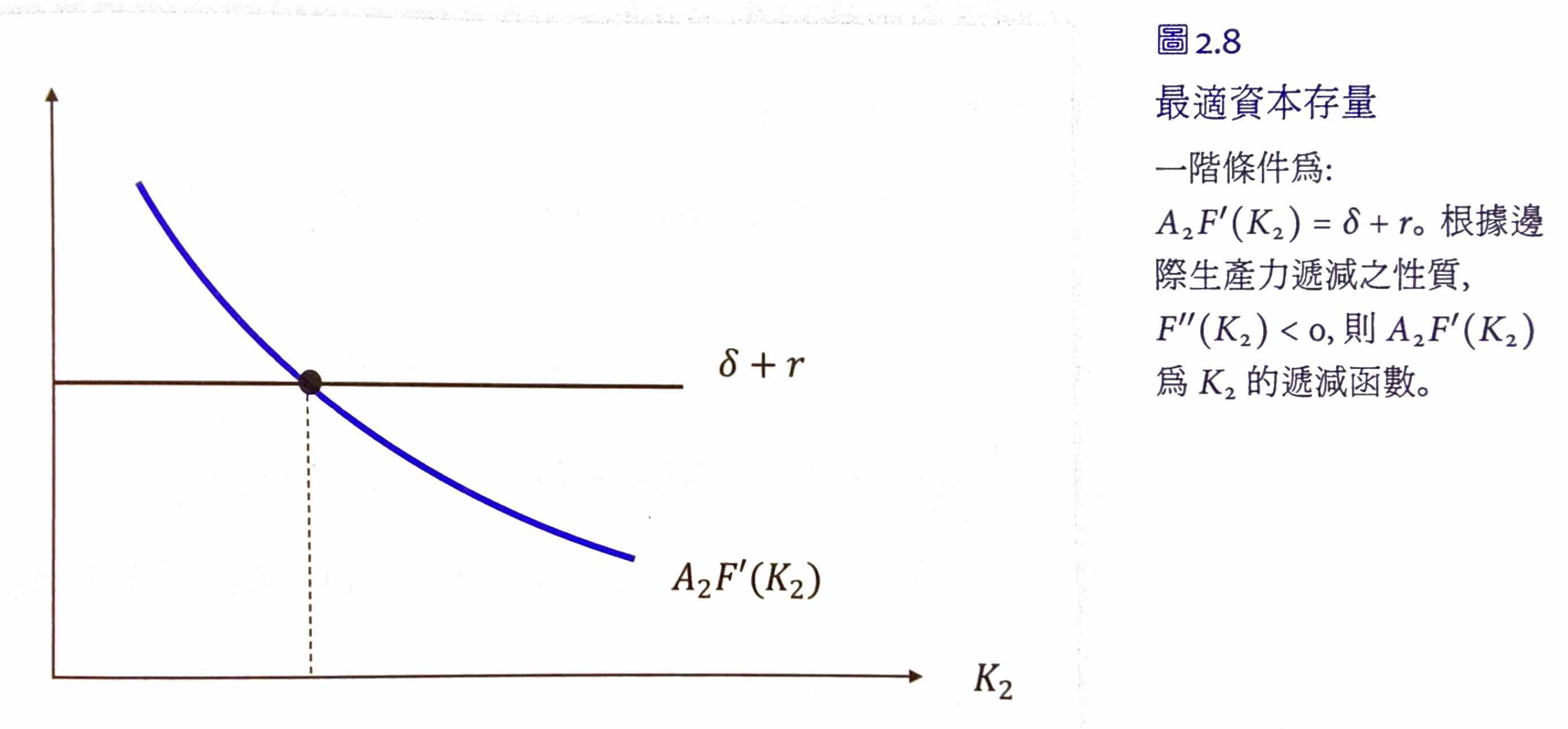
partial \(K_2\)

\[\beta u'(C_2)[A_2F'(K_2)+(1-\delta)-(1+r)]=0\]

Now we know

\[u'(C_1)=\beta u'(C_2)(1+r)=0\]

\[A_2F'(K_2)=\delta+r\]

since \(F''(K_2)<0\), \(K_2\) increases when

• \(A_2\) increases
• \(\delta\) decreases
• \(r\) decreases

Assume \(r=\rho\)

Assume \(K_1=K_2=K\)

If 恆常正向技術衝擊 \(dA_1=dA_2=dA>0\)

• \(\dfrac{dCA_1}{dA}=-\dfrac{F'(K_2)}{A_2F''(K_2)}dA<0\)
• 當期投資增加 -> current account 減少

If 短暫正向技術衝擊 \(dA_1>dA_2=0\)

• \(\dfrac{dCA_1}{dA_1}>0\)
• 當期產出增加 > 當期消費增加 -> current account 增加

If 預期未來正向技術衝擊 \(dA_2>dA_1=0\)

• \(\dfrac{dCA_2}{dA_2}=-\dfrac{dC_1}{dA_2}-\dfrac{dI_1}{dA_2}=<0\)
• 當期投資 & 消費增加 -> current account 減少

Infinite Horizon Intertemporal Current Account Model

See Macroeconomics#世代家庭決策模型

\[U_t=\sum_{s=t}^{\infty} \beta^{s-t}u(C_{s})\]

\[\max_{\{B_{S+1}\}^\infty_{s=t}}\sum_{s=t}^{\infty} \beta^{s-t}u(Y_s+(1+r)B_s-B_{s+1})\]

first-order condition

\[u'(C_s)=(1+r)\beta u'(C_{s+1})\]

no-ponzi-game condition

\[\lim_{T\rightarrow \infty}(\dfrac{1}{1+r})^T B_{t+T-1}\geq 0\]

but no need B in the final period so

橫截條件 transversality condition

\[\lim_{T\rightarrow \infty}(\dfrac{1}{1+r})^T B_{t+T-1}= 0\]

lifetime budget constraint

\[\sum_{s=t}^\infty(\dfrac{1}{1+r})^{s-t}C_s=(1+r)B_t+\sum_{s=t}^\infty(\dfrac{1}{1+r})^{s-t}Y_s\]

Assuming the growth rate of endowment = \(g\) i.e. \(Y_{t+1}=g\cdot Y_t\), then

\[\sum_{s=t}^\infty(\dfrac{1}{1+r})^{s-t}Y_s=\sum_{s=t}^\infty(\dfrac{1+g}{1+r})^{s-t}Y_t\]

So \(g<r\) otherwise the sum of endowment will be infinite, which is meaningless

Assume \(r=\rho\) and \(Y_{t+1}=g\cdot Y_t\)

\[C_t=C_{t+1}\space \forall t$$ $$\begin{align*} & \sum_{s=t}^\infty(\dfrac{1}{1+r})^{s-t}C_s=\dfrac{1+r}{r}C_t\\ &= (1+r)B_t+\sum_{s=t}^\infty(\dfrac{1}{1+r})^{s-t}Y_s\\ &= (1+r)B_t+\sum_{s=t}^\infty(\dfrac{1+g}{1+r})^{s-t}Y_t\\ &= (1+r)B_t+\dfrac{1+r}{r-g}Y_t \end{align*}\]

\[\begin{align*} & CA_t=Y_t+rB_t-C_t\\ &= Y_t-\dfrac{r}{r-g}Y_t\\ &= \dfrac{-g}{r-g}Y_t<0 \end{align*}\]

Meaning if a country keeps growing with the rate of \(g\), there will be an ever-growing current account deficit

\[CA_{t+j}=\dfrac{-g}{r-g}Y_{t+j}=\dfrac{-g}{r-g}(1+g)^jY_t<0\]

The proportion of debt to income will never become 0, explained below

\[\gamma_t=\dfrac{B_t}{Y_t}\]

\[\gamma_{t+1}=\dfrac{B_{t+1}}{(1+g)Y_t}\]

\[\begin{align*} & CA_{t}=\dfrac{-g}{r-g}Y_{t}=B_{t+1}-B_t\\ &= [(1+g)\gamma_{t+1}+\gamma_t]Y_t \end{align*}\]

\[\gamma_t=\dfrac{1}{1+g}\gamma_t-\dfrac{g}{(1+g)(r-g)}\]

Assume \(\gamma_t=\gamma_{t+1}=\bar{\gamma}\)

\[\bar{\gamma}=\dfrac{-1}{r-g}<0\]

Ch3 Uncertainty and Current Account

risk aversion

absolute risk aversion = \(-\dfrac{u''(C)}{u'(C)}\)

relative risk aversion = \(-\dfrac{u''(C)C}{u'(C)}\)

two-period endowment model with uncertainty

當期確定

\[C_1+B_2=Y_1\]

下一期不確定

\[C^H_2=Y^H_2+(1+r)B_2\]

\[C^L_2=Y^L_2+(1+r)B_2\]

lifetime

\[C_1+\dfrac{C^{H/L}_2}{1+r}=Y_1+\dfrac{Y_2^{H/L}}{1+r}\]

according to 當期資訊的 expected 下期 consumption

\[E_1(C_2)=\pi C^H_2+(1-\pi) C^L_2\]

optimization problem

\[\max_{C_1,C_2}u(C_1)+\beta E_1[u(C_2)]\]

Knowing \(C^{H/L}_2=\text{something}-(1+r)C_1\), we can get the first order condition -> stochastic Euler function

\[u'(C_1)=\beta(1+r)E_1[u'(C_2)]\]

\[Var_1(C_2)=E_1(C_2-E_1(C_2))^2\]

謹小慎微 prudence

when \(u'(\cdot)\) is convex i.e. \(u''<0\) & \(u'''>0\)

if \(u'''>0\), then \(C_1<C^{CE}_1\) -> reduce consumption, do precautionary saving

CE = certainty equivalent i.e. having the same expected value as the risk combination but without risk

A prudent person will have a higher saving i.e. current account when facing uncertainty

\[CA_1=Y_1-C_1>Y_1-C^{CE}_1=CA^{CE}_1\]

Simplistic example

• \(u(C)=ln C\)
• \(E(C_2)=\dfrac{1}{2}((C_1-a)+(C_1+a))=C_1\)
• \(u'(C_1)=\dfrac{1}{C_1}<\dfrac{1}{2}(u'(C_1-a)+u'(C_1+a))=\dfrac{C_1}{(C_1-a)(C_1+a)}\)
• so by moving a bit of \(C_1\) to \(C_2\), your utility will increase, meaning there is an incentive for precautionary saving

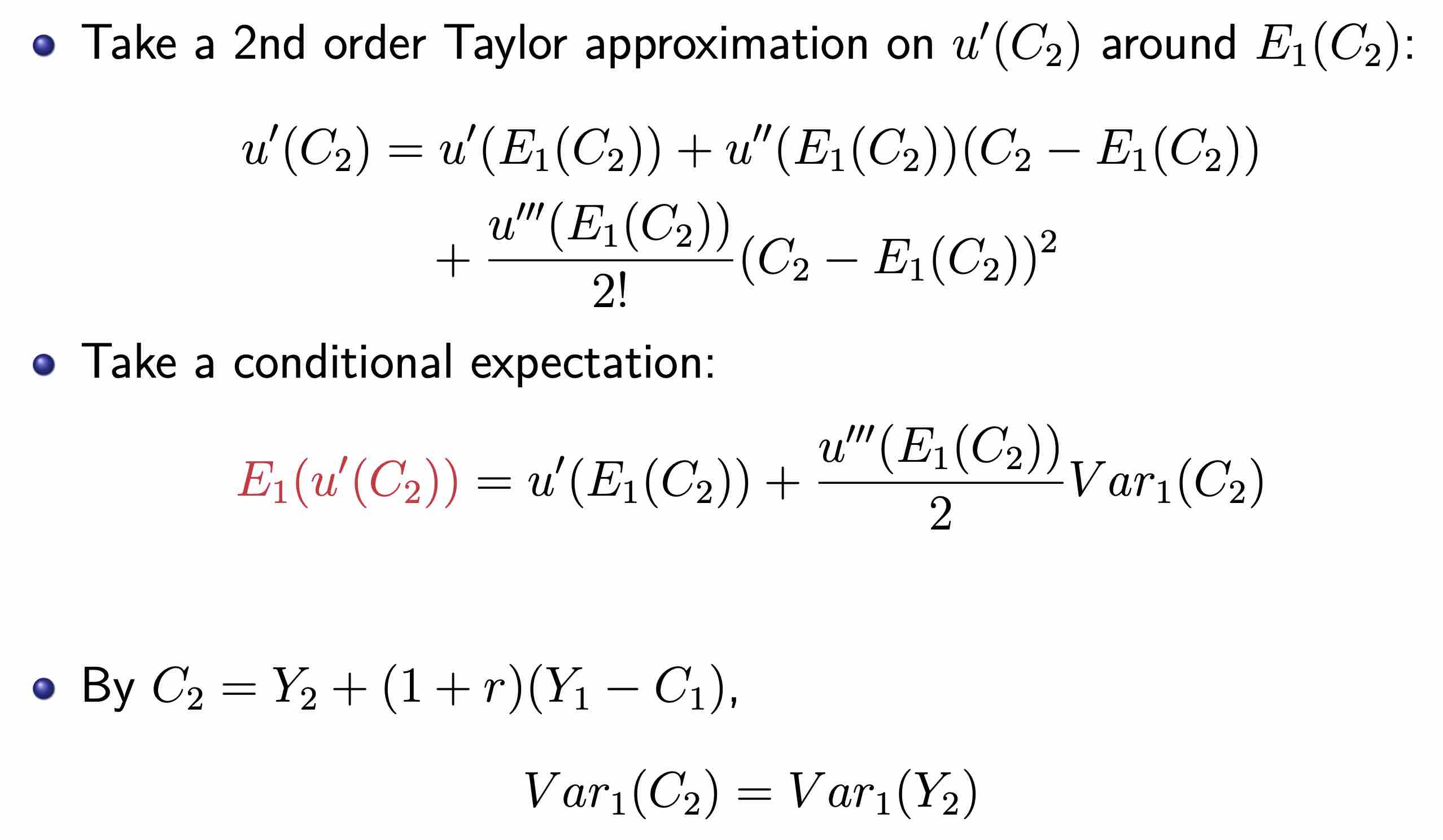
facing normal distribution

Assume

• \(u(C)=-e^{-aC}, a<0\)
  • a prudent utility function
• \(Y_2\) is a normal distribution
  • \(C_2=Y_2+(1+r)(Y_1-C_1)\)
  • \(C_2\) is also a normal distribution

stochastic Euler function

\[u'(C_1)=\beta(1+r)E_1[u'(C_2)]\]

\[e^{-aC_1}=\beta(1+r)E_1(e^{-aC_2})\]

Assume \(r=\rho\)

We know if \(X\) is a normal distribution, then \(E(e^{bX})=e^{\mu b+\frac{1}{2}\sigma^2b^2}\), so

\[e^{-aC_1}=e^{-aE_1(C_2)+\frac{1}{2}a^2Var_1(C_2)}\]

\[C_1=E_1(C_2)-\frac{a}{2}Var_1(C_2)\]

lifetime budget constraint

\[\begin{align*} & C_1+\dfrac{C_2}{1+r}=E_1(C_2)-\frac{a}{2}Var_1(C_2)+\dfrac{C_2}{1+r}\\ &= Y_1+\dfrac{Y_2}{1+r} \end{align*}\]

take expected value

\[E_1(C_2)-\frac{a}{2}Var_1(C_2)+\dfrac{E(C_2)}{1+r}=Y_1+\dfrac{E(Y_2)}{1+r}\]

\[E_1(C_2)=\dfrac{(1+r)Y_1+E_1(Y_2)}{2+r}+\dfrac{a(1+r)}{2(2+r)}Var_1(Y_2)\]

\[\begin{align*} & C_1=E_1(C_2)-\frac{a}{2}Var_1(C_2)\\ &= \dfrac{(1+r)Y_1+E_1(Y_2)}{2+r}-\dfrac{a}{2(2+r)}Var_1(Y_2) \end{align*}\]

no variance for certainty equivalent

\[C^{CE}_1=\dfrac{(1+r)Y_1+E_1(Y_2)}{2+r}\]

precautionary saving

\[C^{CE}_1-C_1=\dfrac{a}{2(2+r)}Var_1(Y_2)\]

two-period endowment model with production & investment with uncertainty

If \(A_2\) & \(u'(C_2)\) are independent, then \(K_2=K^{CE}_2\)

If \(Cov_1(A_2, C_2)>0\) -> \(Cov_1(A_2, u'(C_2))<0\), then \(K_2<K^{CE}_2\) i.e. reduce investment

current account

\[\begin{align*} & CA_1=B_2-B_1=B_2\\ &= A_1F(K_1)-C_1-K_2 \end{align*}\]

When there is uncertainty in period 2, \(C_1<C^{CE}_1\) & \(K_2<K^{CE}_2\), meaning a bigger current account

\[CA_1>CA^{CE}_1\]

Ch4 Foreign Exchange Market Intro

quotes

direct quotes

1 unit of foreign currency -> ? units of home currency

\[S^{H/F}=\dfrac{\text{Home Currency}}{\text{Foreign Currency}}\]

American quotes \(S^{US/F}\) = direct quotes for USD

indirect quotes

1 unit of home currency -> ? units of foreign currency

\[S^{F/H}=\dfrac{\text{Foreign Currency}}{\text{Home Currency}}\]

European quotes \(S^{F/US}\) = indirect quotes for USD

cross rate

cross rate = a quote not involving USD but 2 other currencies

triangular arbitrage

if A/C = A/B x B/C then there's not triangular arbitrage

外匯交易類型

market type

• spot market 現貨市場
  • <= 2d 交割
  • uses spot rate 即期匯率
  • normally 匯率 refers to spot rate
• forward market 遠期外匯市場
  • at a specific future date

price

• bid price 買價
  • the price the bank buys at
• ask price 賣價
  • the price the bank sells at
• bid-ask spread = ask price - bid price
• factors affecting bid-ask spread
  • cost
    • smaller 交易 cost -> smaller bid-ask spread
  • risk
    • higher risk -> larger bid-ask spread
  • market thickness
    • smaller market -> less liquidity -> higher risk -> larger bid-ask spread

匯率變動

匯率

\[S_t=S^{H/F}=\dfrac{\text{Home Currency}}{\text{Foreign Currency}}\]

foreign currency appreciates -> \(S_t\) up

匯率變動

\[\dfrac{S_{t+1}-S_t}{S_t}=\dfrac{\Delta S_{t+1}}{S_t}\]

e.g. 1 foreign = 20 home -> 1 foreign = 30 home, then foreign currency appreciation rate = 50%

Note that foreign currency appreciation rate != home currency depreciation rate. We can use log-difference to solve this problem.

\[\begin{align*} & \Delta \log S_{t+1}=\log S_{t+1}-\log S_{t}\\ &= -\left(\log \dfrac{1}{S_{t+1}}-\log\dfrac{1}{S_t}\right) \end{align*}\]

first-order Taylor approximation

given \(\log(1+g_t)\approx g_t\)

\[\dfrac{S_{t+1}-S_t}{S_t}\approx\log\left(1+\dfrac{S_{t+1}-S_t}{S_t}\right)=\log S_{t+1}-\log S_t\]

continuously compounded rate

\(g_{t+1}\) = foreign currency appreciation rate in a year, \(d_{t+1}\) = continuously compounded rate in a year

If we divide a year into \(n\) period for compounded rate

\(S_{t+1}=S_t\left[1+\left(\dfrac{d_{t+1}}{n}\right)^n\right]\)

We know \(\lim_{n\rightarrow\infty}\left[1+\left(\dfrac{d_{t+1}}{n}\right)^n\right]=e^{d_{t+1}}\)

So

\[S_{t+1}=S_te^{d_{t+1}}\]

\[d_{t+1}=\log S_{t+1}-\log S_t\]

multilateral exchange rate

geometric weighted average of exchange rate to multiple currencies, with weight = trade amount

EER effective exchange rate i.e. multilateral exchange rate

\[EER=\prod_{i=1}^n\left(\dfrac{1}{S_i}\right)^{w_i}, \sum_i^nw_i=1\]

\[\dfrac{1}{EER}=\prod_{i=1}^n\left(S_i\right)^{w_i}\]

• \(\dfrac{1}{S_i}\) = indirect quote to country \(i\)
• \(w_i\) = ratio of trade to country \(i\) to total trade amount

average change rate

\[\Delta\log EER=\sum_{i=1}^n w_i\Delta \log\dfrac{1}{S_i}\]

有效匯率指數=\(\dfrac{EER_t}{EER_0}\times 100\)

• EER at period t / EER at base period
• up when NTD appreciates against a basket

foreign exchange derivatives

• forwards 遠期外匯
  • trade in the future
  • can't be traded in secondary market
• swaps 換匯交易
  • a contract to trade now and trade back later
• futures 外匯期貨
  • trade in the future
  • can be traded in secondary market
• options 外匯選擇權
  • an option to trade in the future

foreign exchange reserves

official international reserves includes

• foreign exchange reserves
• gold reserves
• IMF-related reserve assets
  • Taiwan's not in IMF so not for Taiwan

optimal foreign exchange reserves

• 3-6 months of import
• 100% short term debt
• 20% M2

However, Taiwan's foreign exchange reserves >> the optimal point

Before 1987, Taiwan's private banks are forbidden to have foreign exchange, so they're all sold to the central bank.

Ch5 Exchange rate

exchange rate regime

Ch17 貨幣政策的目標機制

how central banks control the exchange rate

theoretical

• free floating
  • zero intervention
• managed floating
  • dirty floating
  • central bank intervenes frequently
• fixed rate
  • fixed to a big currency e.g. USD EUR or a basket of currencies

de facto

IMF's report

• hard pegs
  • no separate legal tender
    • use a major currency as its own
    • called Dollarization if use USD
  • currency board
    • fixed exchange rate to a major currency
• soft pegs
  • conventional peg
    • target at a currency or a basket
  • stabilized arrangement
    • within 2% of change within 6 months
    • TW probably this
  • crawling peg
    • constant rate of change
  • crawl-like arrangement
    • within 2% of change in the rate of change
  • pegged exchange rate within horizontal bands
    • target at a zone
• floating regime
  • floating
    • intervene only to slow down the rate of change
  • free floating
    • almost never intervene

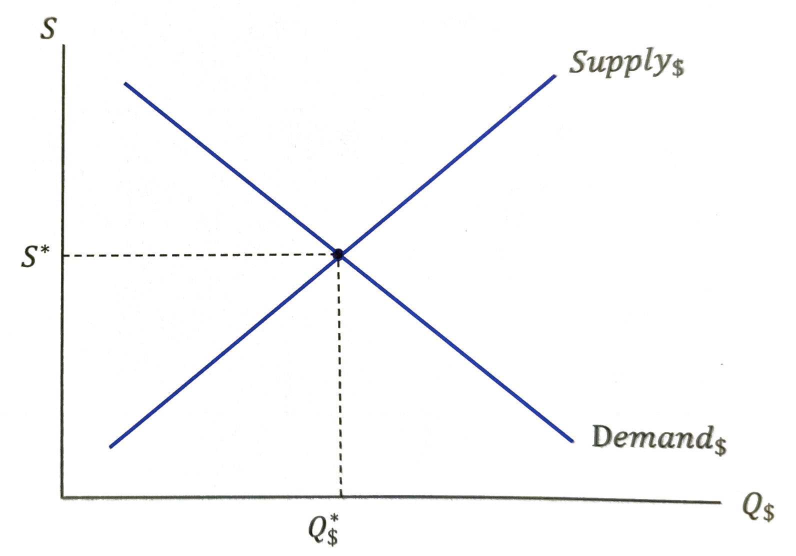
equilibrium

the foreign exchange market of USD, direct quote (TWD/USD) vs. quantity

• supply from exporters
  • sell and get USD
• demand from importers
  • need USD to pay

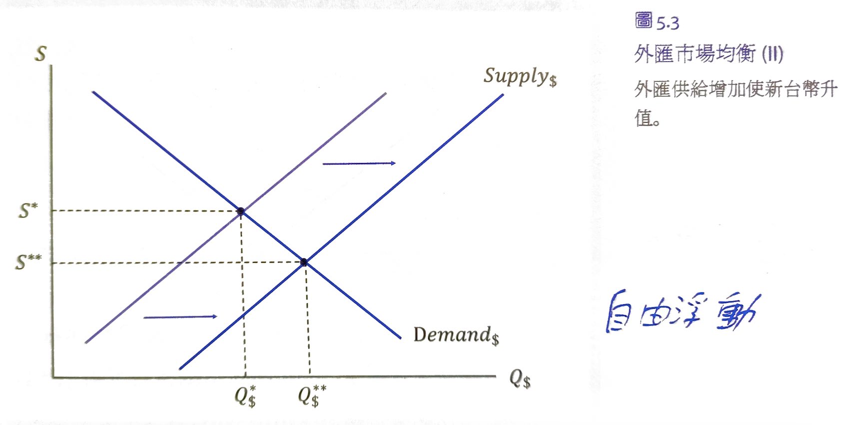
free floating

export up -> supply shifts right -> S down i.e. TWD appreciates

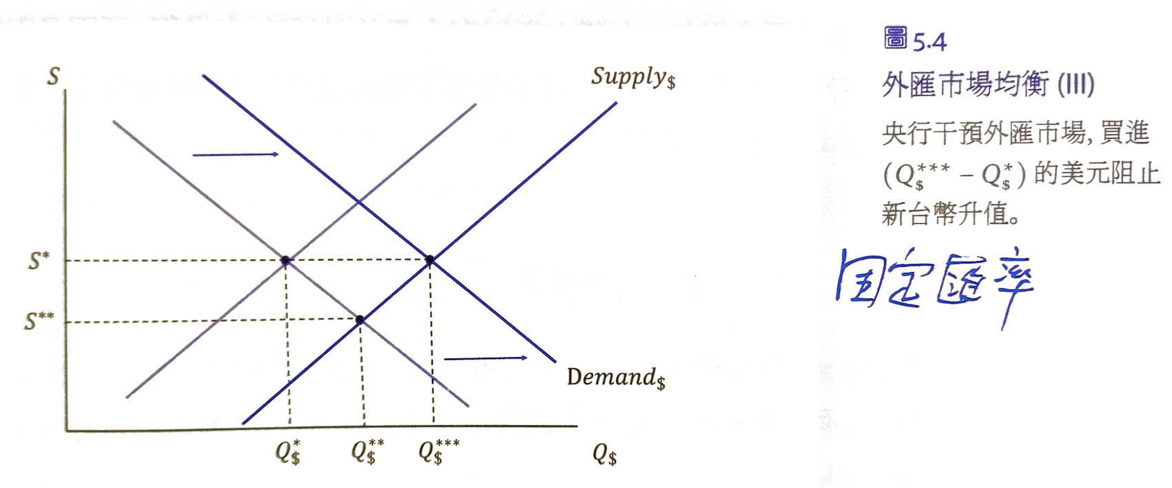
fixed rate

export up -> supply shifts right -> central bank intercepts by buying \((Q^{***}-Q^*)\) of USD -> demand shifts right -> S unchanged

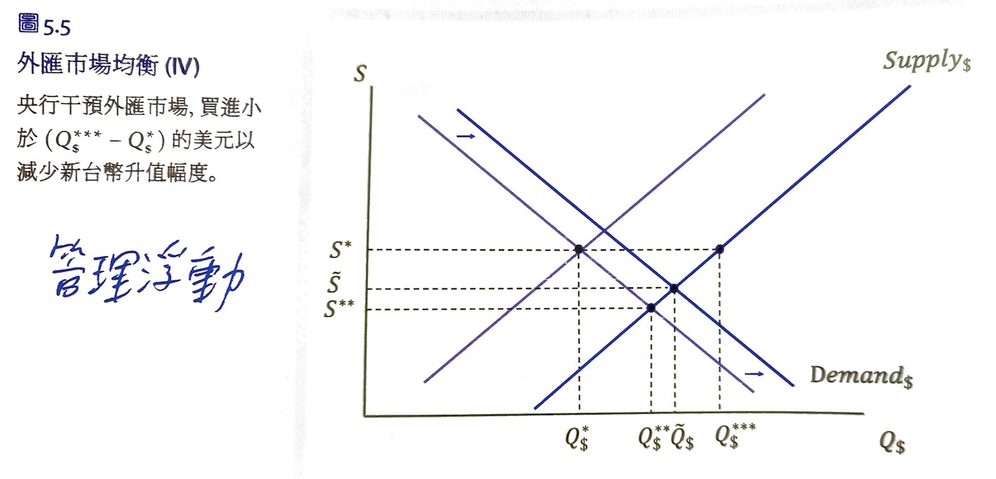
managed floating

export up -> supply shifts right -> central bank buys some USD -> demand shifts right a bit -> S reduced a bit

risk of exchange rate

Since exchange rate is a random walk, there is risk in transactions involving different currencies.

without random shocks

\[S_t=f(D_t,S_t)\]

with random shocks

\[S_t=f(D_t+\epsilon_{1t},S_t+\epsilon_{2t})+\epsilon_{3t}\]

where \(\epsilon_{jt}=\rho_j\epsilon_{jt-1}+v_{jt}\), \(\rho_j\) is a constant, \(v_{jt}\sim^{i.i.d.}(0,\sigma_j^2)\), \(j=1,2,3\)

\(\epsilon_{1t}\), \(\epsilon_{2t}\), and \(\epsilon_{3t}\) are random processes, making \(S_t\) a random process as well

time series analytics

logrithmic difference

Given Taylor approximation, when \(\Delta y_t\) is small

\[\dfrac{y_{t}-y_{t-1}}{y_{t-1}}\approx\log\left(1+\dfrac{y_{t}-y_{t-1}}{y_{t-1}}\right)=\log(y_t)-\log(y_{t-1})=\Delta y_t\]

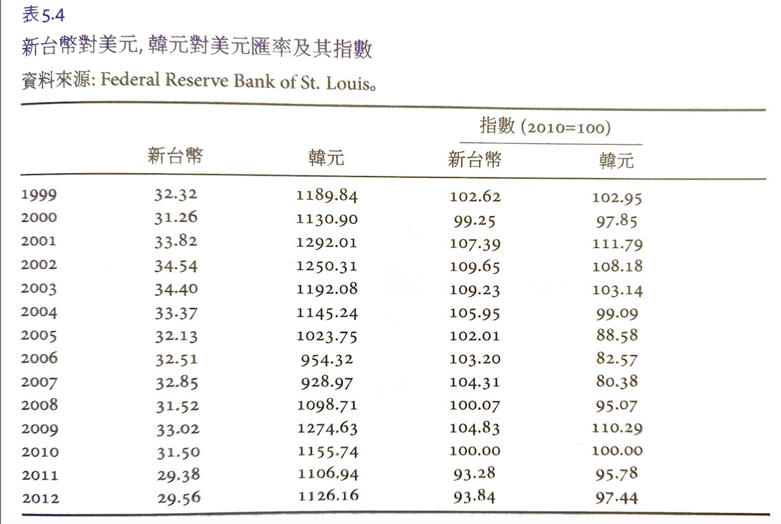
base period normalization

Set a base period and normalize all values with base period being 100 for ease of comparison.

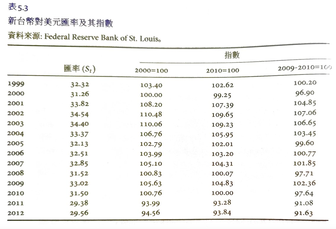
2009-2010 means using mean of 2009 & 2010 as 100

empirical analysis

exchange rate change \(r_t\)

\[r_t=\dfrac{S_t-S_{t-1}}{S_t}\times 100\sim N(0,\sigma^2)\]

PDF of \(r_t\) of GBP vs. USD

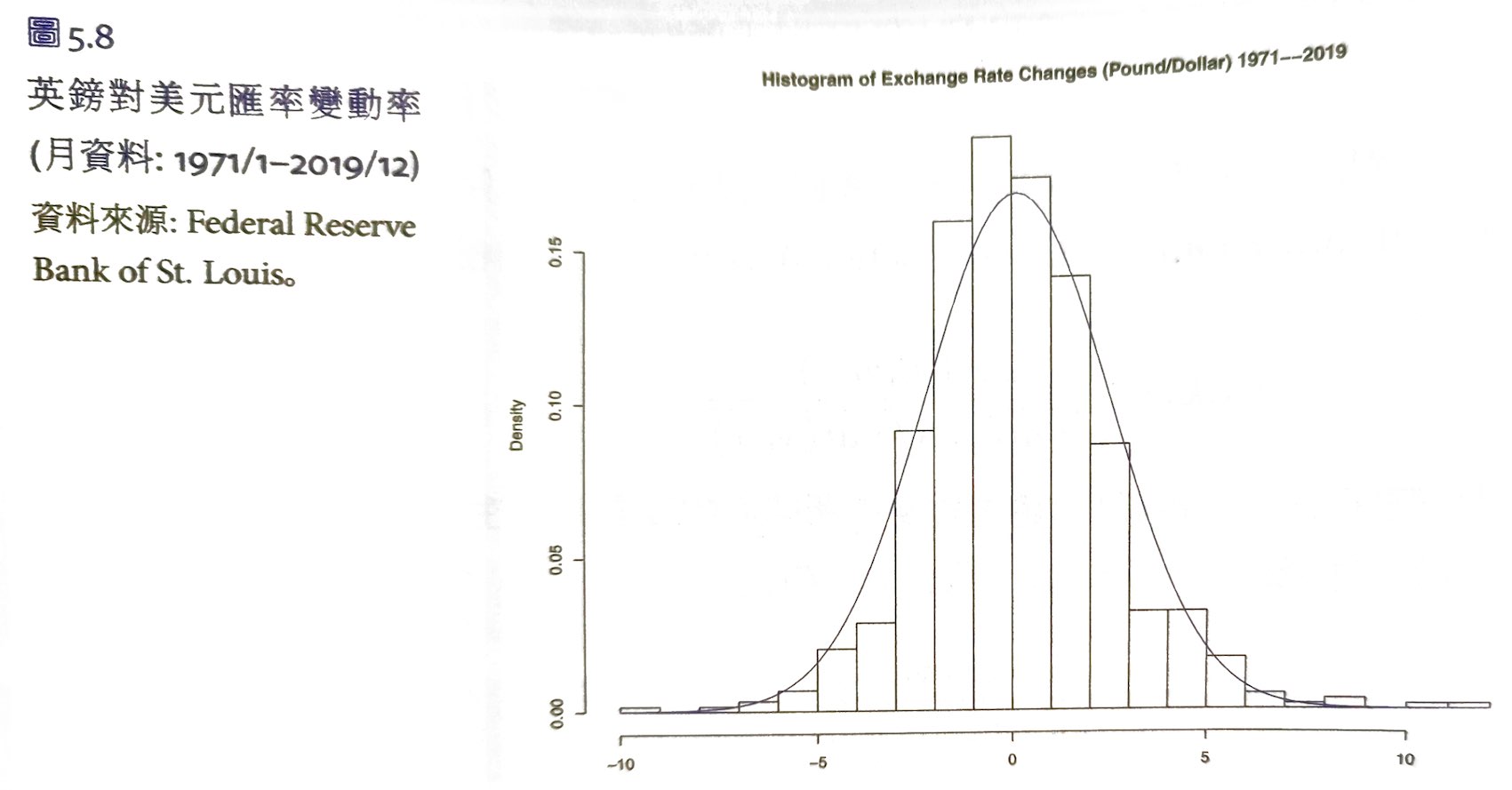
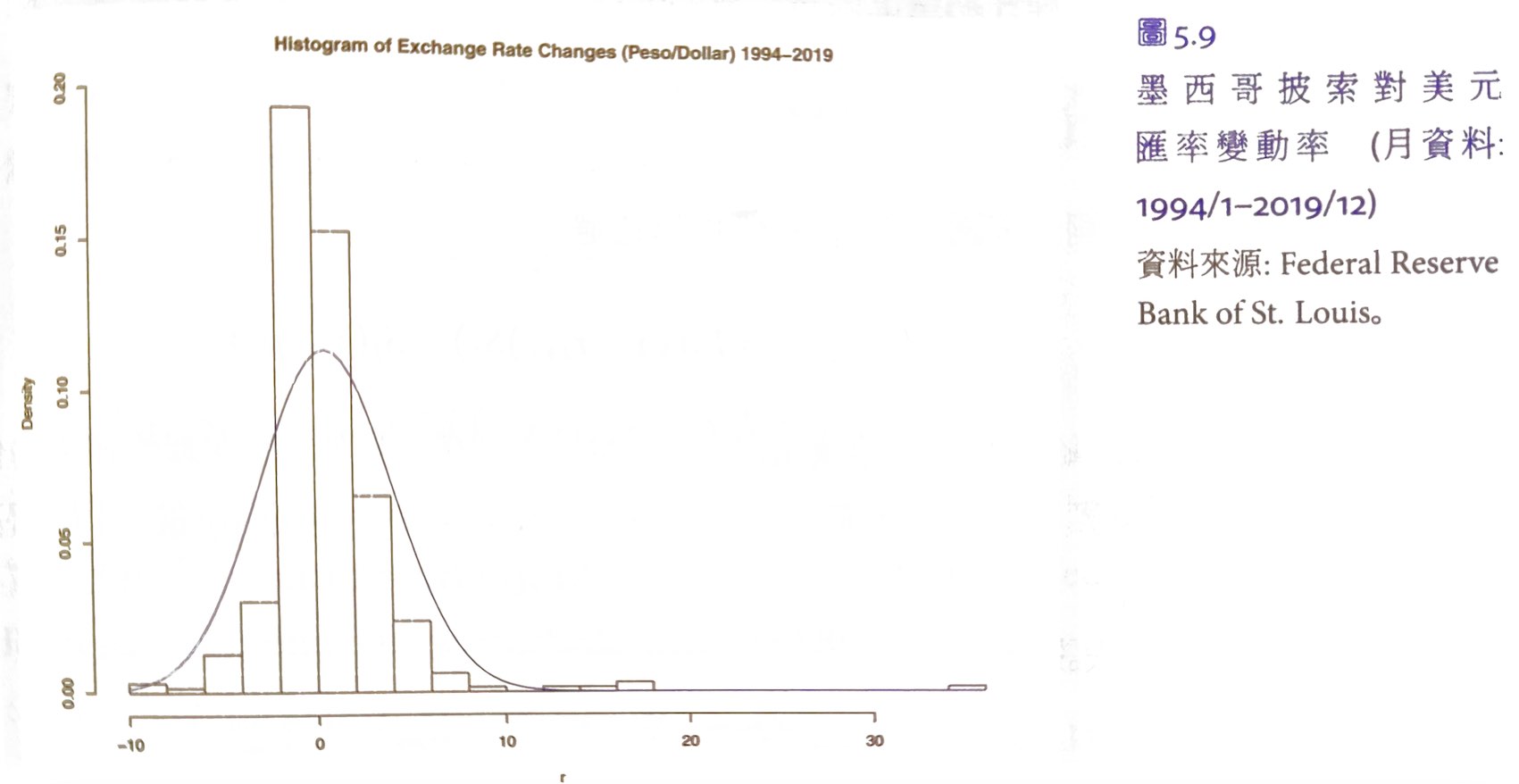
In emerging market countries, however, \(r_t\) is not a normal distribution.

PDF of \(r_t\) of MXN vs. USD is right-skewed, meaning the probability of depreciation is higher.

expected exchange rate

\[\mu_t=E_t(r_{t+1})\]

\[E_t(S_{t+1})=E_t((1+r_{t+1})S_t)=S_t(1+\mu_t)\]

\(X_{jt}\) are variables effecting the foreign exchange market

\[\hat{\mu}_t=\hat{\alpha}+\sum\hat{\beta_j}X_{jt}\]

\[\hat{S}_{t+1}={S}_t(1+\hat{\mu}_t)\]

hedge

Can use forward exchange contract to eliminate risk: a contract to buy/sell X foreign currency at the exchange rate \(F\) in the future. See #Ch6 Covered Interest Rate Parity for in depth analysis.

Example

A TW form will get 1M USD a year later. Given current exchange rate = 29.5 TWD/USD, USD interest rate = 6%, TWD interest rate = 10%, what will the forward exchange contract be?

\[1.1=1.06\times\dfrac{F}{29.5}\]

\[F=30.61\]

So the firm should have a contract to sell 1M USD at 30.61 TWD/USD a year later.

If the actual exchange rate turns out to be 31 TWD/USD, then the firm loses.

Ch6 Covered Interest Rate Parity

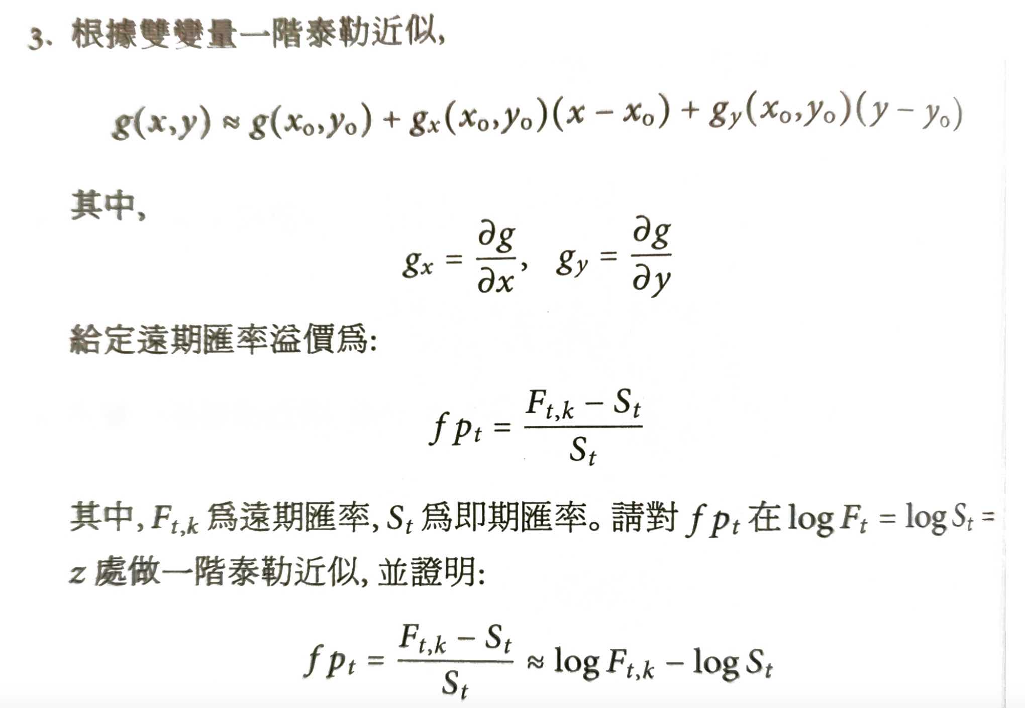
forward premium

forward premium = how much forward exchange rate stray away from current one

\[\begin{align*} & fp_{t,k}=\dfrac{F_{t,k}-S_t}{S_t}\\ & = \dfrac{F_{t,k}}{S_t}-1 \approx \log\dfrac{F_{t,k}}{S_t} = \log F_{t,k}-\log S_t \end{align*}\]

annualized percentage of forward premium of k days = \(fp_{t,k}\dfrac{360}{k}\) (most use 360 days as a year)

covered interest rate parity, CIP

the equilibrium price of forward exchange rate

\[1+i_t=\dfrac{1+i_t^*}{S_t}F_{t,k}\]

• \(i_t\) = k-day interest rate of home country
• \(i_t^*\) = k-day interest rate of foreign country
• \(S_t\) current exchange rate H/F
• \(F_{t,k}\) = k-day forward exchange rate H/F

otherwise there will be opportunity for arbitrage

\[\log F_{t,k}-\log S_t=\log(1+i_t)-\log(1+i^*_t)\approx i_t-i^*_t\]

\[fp_{t,k}\approx \log F_{t,k}-\log S_t\approx i_t-i^*_t\]

i.e. forward premium = interest rate spread between the the home & foreign country

There will be forward premium when foreign country has a lower interest rate and discount if higher.

empirical study of CIP

If CIP is correct, then \(\alpha=0\) & \(\beta=1\)

\[f_{t,k}-s_t=\alpha+\beta(i_t-i_t^*)+\epsilon_t\]

Regression result:

• null hypothesis of \(\alpha=0\) is rejected
• null hypothesis of \(\beta=1\) can't be rejected

\(\alpha \neq 0\) can be explained by

• transaction costs of arbitrage
• default risk
  • contract may turn out to be unfulfilled
• exchange controls
  • cannot freely do arbitrage
• political risk
  • same as exchange controls

forward exchange rate

\[F_t(n)=S_t\left(\dfrac{1+i_t(n)}{1+i^*_t(n)}\right)^n\]

• \(F_t(n)\) = n-year foward exchange rate H/F
• \(i_t\) = 1-year interest rate of home country
• \(i_t^*\) = 1-year interest rate of foreign country
• \(S_t\) current exchange rate H/F

home n-year bonds & exchange -> foreign n-year bonds -> exchange back should have the same reward

problems

Ch7 Foreign Exchange Market Risk

FRU & UIP

forward rate unbiasedness (FRU) hypothesis

\[F_t=E_t(S_{t+1})=E(S_{t+1}|\Omega_t)\]

foward exchange rate = expected future exchange rate

the mean of prediction error = 0

\[u_{t+1}=S_{t+1}-F_t\]

\[E_tu_{t+1}=E(u_{t+1}|\Omega_t)=E(S_{t+1}|\Omega_t)-F_t=0\]

Siegel paradox

\[E_t(\dfrac{1}{S_{t+1}})>\dfrac{1}{E_t(S_{t+1})}=\dfrac{1}{F_t}\]

so FRU can't be true for both home & foreign currency at the same time

However, the disparity isn't very significant, as it still holds Taylor approximation#first-order.

\[\dfrac{1}{S_{t+1}}\approx\dfrac{1}{F_t}+\dfrac{S_{t+1}-F_t}{F_t^2}\]

\[E_t\left[\dfrac{1}{S_{t+1}}\right]\approx\dfrac{1}{F_t}\]

uncovered interest rate parity, UIP

\[1+i_t=\dfrac{1+i_t^*}{S_t}F_{t,k}=\dfrac{1+i_t^*}{S_t}E_t(S_{t+1})\]

\[E_t(1+i_t)=E_t\left(\dfrac{S_{t+1}}{S_t}(1+i_t^*)\right)\]

expected return of home asset = that of foreign asset

Didn't actually buy/sell in forward exchange market to avoid risk so it's "uncovered".

\[E_t\left(\dfrac{S_{t+1}}{S_t}\right)=\dfrac{1+i_t}{1+i_t^*}\]

if home interest rate > foreign interest rate, then foreign currency is expected to appreciate

empirical study of FRU & UIP

They are not true according to empirical data.

It's because foreign investment involves future exchange rate which contains risk, and investors are not risk-neutral, while home investment is risk-free.

CAPM

capital asset pricing model, CAPM

risk premium of risky assets

\[E(R_i)-r_f=\beta(E(R_m)-r_f)\]

\[\beta=\dfrac{Cov(R_i,R_m)}{Var(R_m)}\]

• \(R_m\) = rate of return of market portfolio, a combination of large and well-diversified investment
• \(R_i\) = rate of return of an individual asset
• \(r_f\) = risk-free rate of return i.e. rate of return on risk-free assets

The higher the \(\beta\), the higher the risk premium

For UIP

\[\begin{align*} & E(R^*_{t+1})-r_{f,t+1}=\beta(E_t(R_{m,t+1})-r_{f,t+1})\\ &= \Lambda_tCov(S_{t+1},R_{m,t+1}) \end{align*}\]

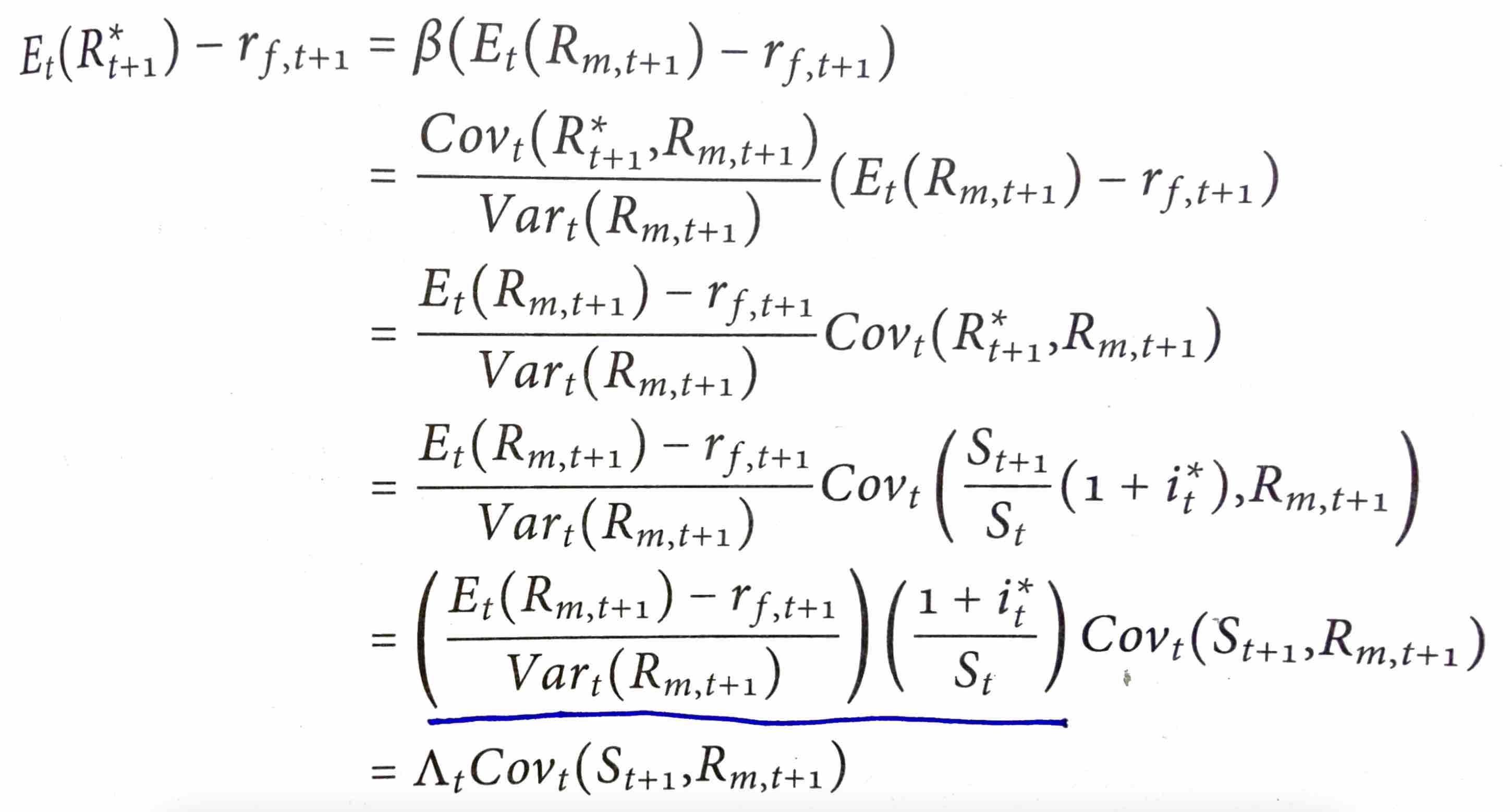
the risk premium of foreign asset is dependent on the covariance of future exchange rate & market rate of return

\[\begin{align*} & E(R^*_{t+1})-r_{f,t+1}\\ &= i^*_t+E_t(\log S_{t+1} - \log S_t)-i_t+\dfrac{1}{2}Var_t(\log S_{t+1})\\ &= \Lambda_tCov(S_{t+1},R_{m,t+1}) \end{align*}\]

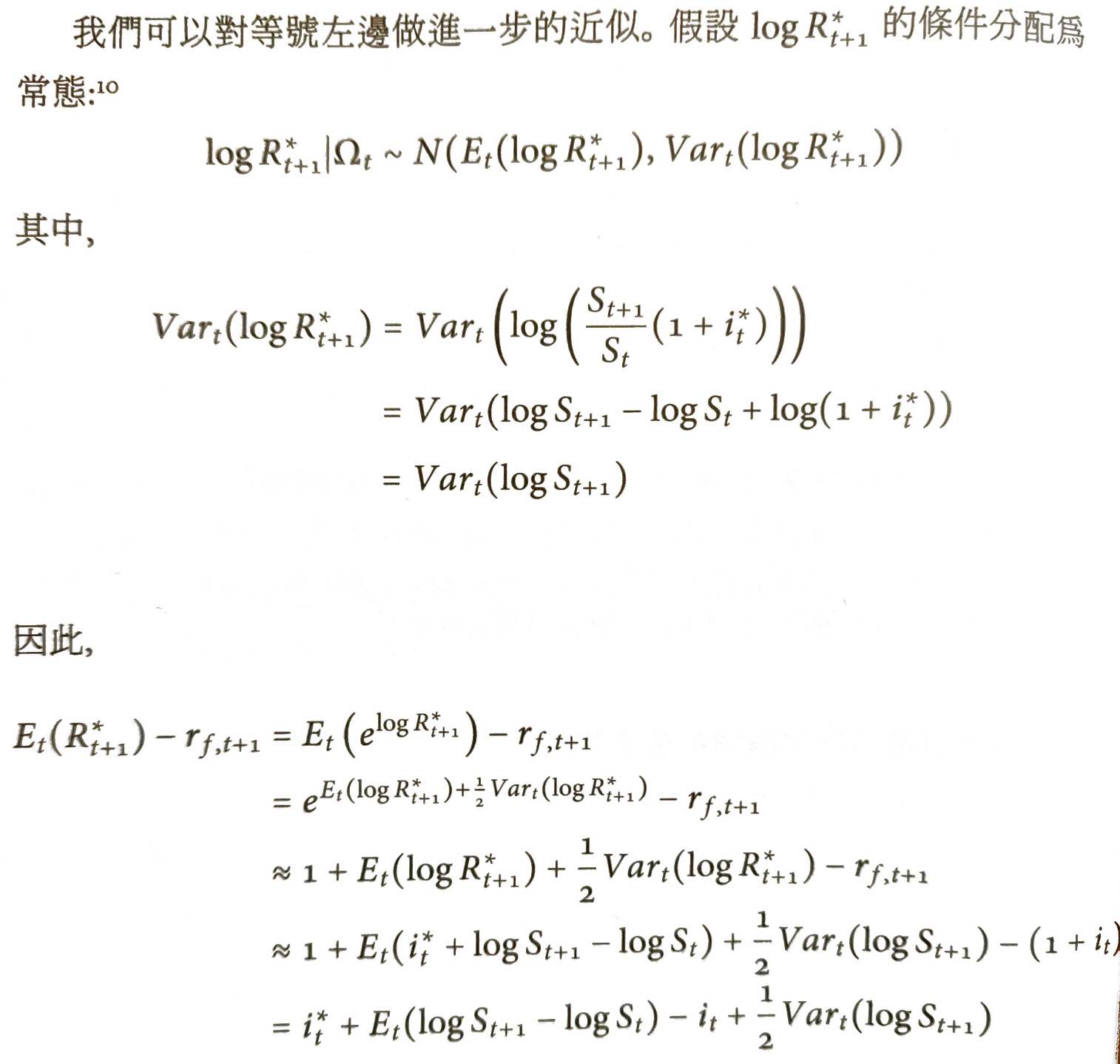
UIP with risk premium

\[\begin{align*} & \rho_t=i^*_t+E_t(\log S_{t+1}-\log S_t)-i_t\\ &= i^*_t+(E_t\log S_{t+1}-\log S_t)-i_t\\ &= -\dfrac{1}{2}Var_t(\log S_{t+1})+ \Lambda_tCov(S_{t+1},R_{m,t+1}) \end{align*}\]

• \(\Lambda_tCov(S_{t+1},R_{m,t+1})\) = marginal risk of CAPM
• \(-\dfrac{1}{2}Var_t(\log S_{t+1})\) = Jensen's Inequality adjustment

\[i^*_t-i_t=\rho_t-(E_t\log S_{t+1}-\log S_t)\]

CCAPM

consumption capital asset pricing model, CCAPM

Assuming

• 2 periods
• small open economy
  • home bonds \(B\) of interest rate \(i\)
  • foreign bonds of interest rate \(i^*\) (in foreign currency)
    • \(B^*\) with forward exchange contract to exchange back to home currency at \(F\)
    • \(\tilde{B^*}\) w/o forward exchange contract
  • \(B_1=B^*_1=\tilde{B}^*_1=0\)
  • \(B_3=B^*_3=\tilde{B}^*_3=0\)
• product
  • consumption quantity \(C_t\)
  • price \(P_t\)
• endowment \(Y_t\)
  • \(Y_1\) at period 1
  • 2 possibilities in period 2
    • \(Y^H_2\) with probability \(\pi\)
    • \(Y^L_2\) with probability \(1-\pi\)

budget constraint

\[P_1C_1+B_2+S_1B^*_2+S_1\tilde{B^*_2}=Y_1\]

\[P^H_2C^H_2=Y^H_2+(1+i)B_2+F_1(1+i^*)B^*_2+S^H_2(1+i^*)\tilde{B^*_2}\]

\[P^L_2C^L_2=Y^L_2+(1+i)B_2+F_1(1+i^*)B^*_2+S^L_2(1+i^*)\tilde{B^*_2}\]

we can rewrite them to make \(C_1,C^H_2,C^L_2\) dependent on \(B_2,B^*_2,\tilde{B}^*_2\)

lifetime utility optimization problem

\[\begin{align*} & \max_{\{B_2,B^*_2,\tilde{B}^*_2\}}U=u(C_1)+\beta E_1[u(C_2)]\\ &= u(C_1)+\beta (\pi u(C^H_2)+(1-\pi)u(C^L_2)) \end{align*}\]

Can get 3 first-order equations by partial against \(B_2,B^*_2,\tilde{B}^*_2\)

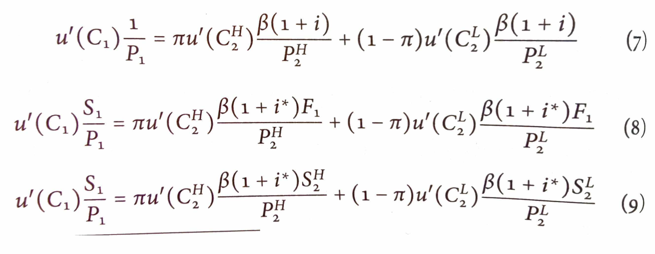
from (7)

\[1=(1+i)E_1\left[\dfrac{\beta u'(C_2)}{u'(C_1)}\dfrac{P_1}{P_2}\right]=(1+i)E_1[M_2]\]

where \(M_2\) is pricing kernel

\[M_2\equiv\dfrac{\beta u'(C_2)}{u'(C_1)}\dfrac{P_1}{P_2}\]

from (8)

\[1=(1+i^*)\dfrac{F_1}{S_1}E_1\left[\dfrac{\beta u'(C_2)}{u'(C_1)}\dfrac{P_1}{P_2}\right]=(1+i^*)\dfrac{F_1}{S_1}E_1[M_2]\]

meaning

\[1+i=\dfrac{F_1}{S_1}(1+i^*)\]

which is #covered interest rate parity, CIP

from (9)

\[1=(1+i^*)E_1\left[\dfrac{S_2}{S_1}\dfrac{\beta u'(C_2)}{u'(C_1)}\dfrac{P_1}{P_2}\right]=(1+i^*)E_1\left[\dfrac{S_2}{S_1}M_2\right]\]

meaning

\[F_1=\dfrac{E_1[S_2M_2]}{E_1[M_2]}=\dfrac{E_1[S_2]E_1[M_2]+Cov_1(S_2,M_2)}{E_1[M_2]}\]

\[1+i=\dfrac{(1+i^*)}{S_1}\dfrac{E_1[S_2M_2]}{E_1[M_2]}=\dfrac{(1+i^*)}{S_1}\dfrac{E_1[S_2]E_1[M_2]+Cov_1(S_2,M_2)}{E_1[M_2]}\]

when \(Cov_1(S_2,M_2)\) = 0, \(F_1=E_1[S_2]\) and \((1+i)=(1+i^*)\dfrac{E_1[S_2]}{S_1}\) i.e. #FRU & UIP is true

\[\dfrac{(1+i)S_1}{(1+i^*)E_1[S_2]}=\dfrac{Cov_1(S_2,M_2)}{E_1[M_2]E_1[S_2]}+1\]

\[\log(1+i)+\log(S_1)-\log(1+i^*)-\log(E_1[S_2])=\log\left(\dfrac{Cov_1(S_2,M_2)}{E_1[M_2]E_1[S_2]}+1\right)\]

\[i+\log(S_1)-i^*-E_1[\log S_2]=\dfrac{Cov_1(S_2,M_2)}{E_1[M_2]E_1[S_2]}\]

risk premium of foreign asset \(\rho\)

\[\rho=i^*+E_1[\log S_2]-\log(S_1)-i=-\dfrac{Cov_1(S_2,M_2)}{E_1[M_2]E_1[S_2]}\]

if \(Cov_1(S_2,M_2)<0\): \(C_2\) down -> \(u'(C_2)\) up -> \(M_2\) up -> \(S_2\) down i.e. home currency appreciates -> foreign asset return down, so risk premium \(\rho>0\) naturally as it contains higher risk

\[i+\rho=i^*+E_1[\log S_2]-\log(S_1)\]

other explanations of UIP being wrong

• investors are not rational
• Peso problem
  • investors also consider the possibility of black swan events, which the real data we run regression on do not contain these kind of events
• foreign exchange market is not efficient
  • big investors are efficient but small ones are not

problems

P4

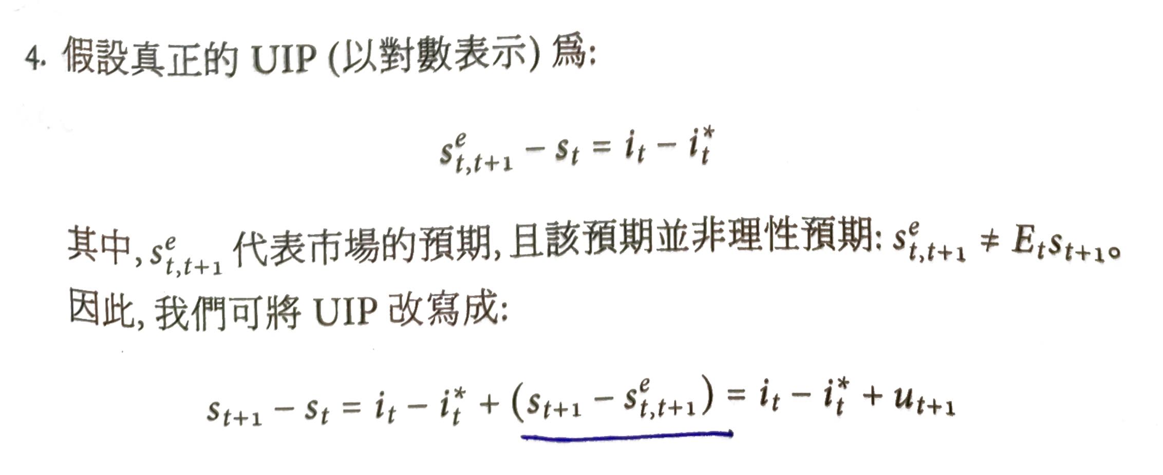
(a)

• \(A=i_t-i^*_t\)
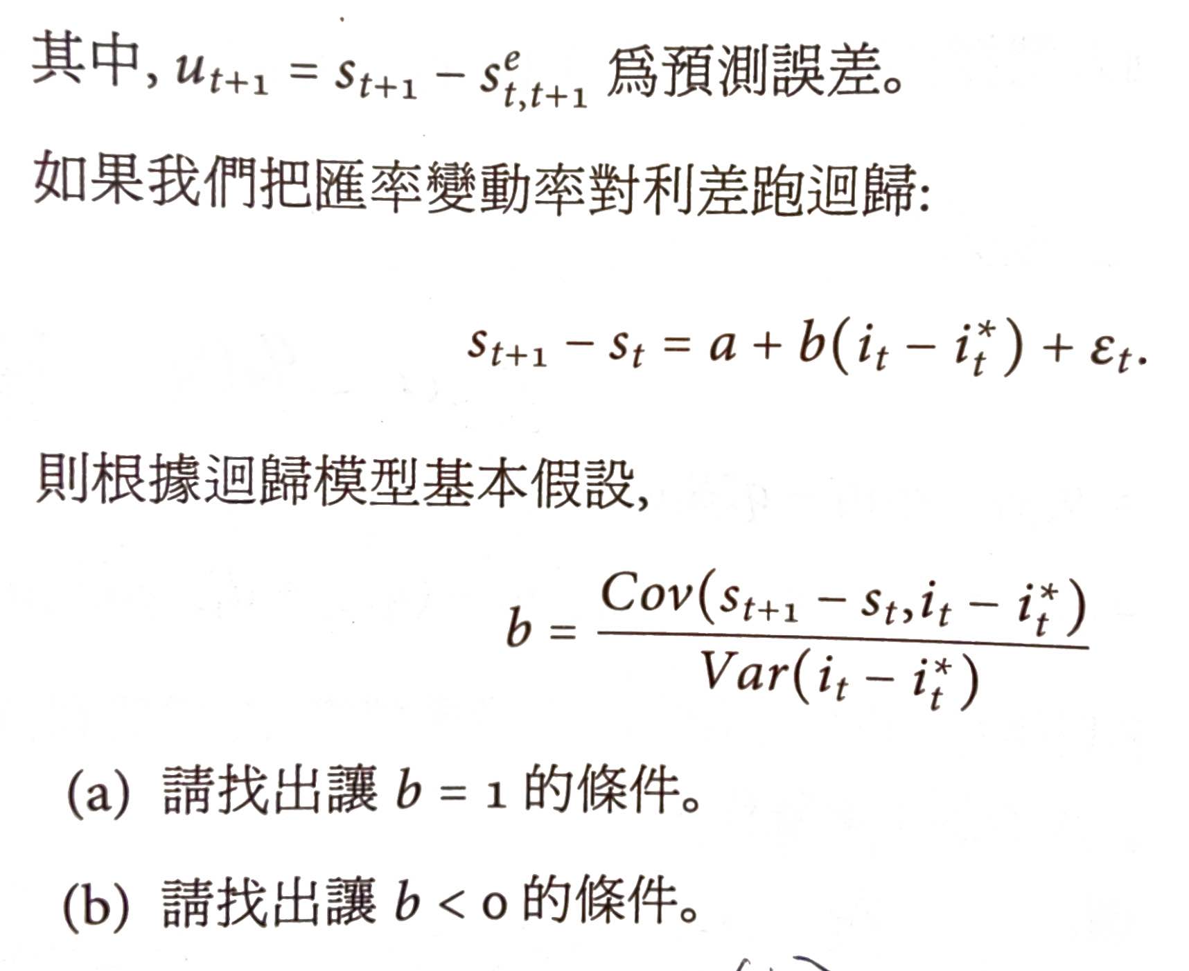
• \(B=u_{t+1}\)
• \(s_{t+1}-s_t=A+B\)
• \(Cov(x,y)=E[xy]-E[x]E[y]\)
• \(Var(x)=E[x^2]-E[x]^2\)

For \(b=1\), \(Cov(A+B,B)=Var(A)\)

\[\begin{align*} & Cov(A+B,A)=E[(A+B)A]-E[A+B]E[A]\\ &= E[A^2]-E[A]^2+E[AB]-E[A]E[B]\\ &= Var(A)+Cov(A,B) \end{align*}\]

So if \(Cov(A,B)=Cov(i_t-i^*_t,u_{t+1})=0\), \(b=1\)

(b)

For \(b<0\), \(Cov(A+B,B)=Var(A)+Cov(A,B)<0\)

So \(Cov(A,B)=Cov(i_t-i^*_t,u_{t+1})<-Var(a)=-Var(i_t-i^*_t)\)

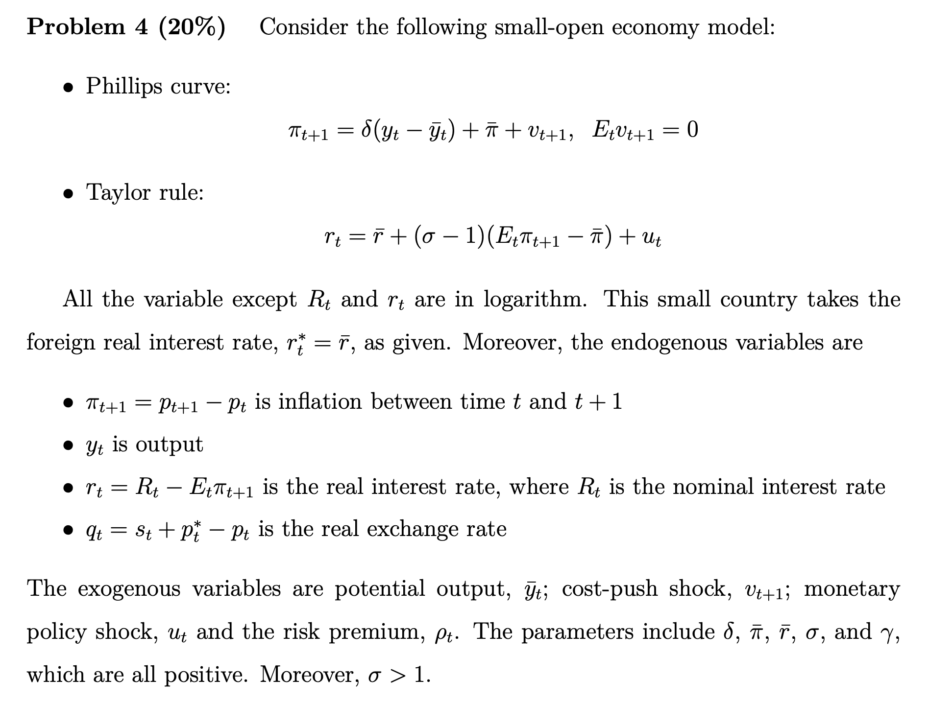
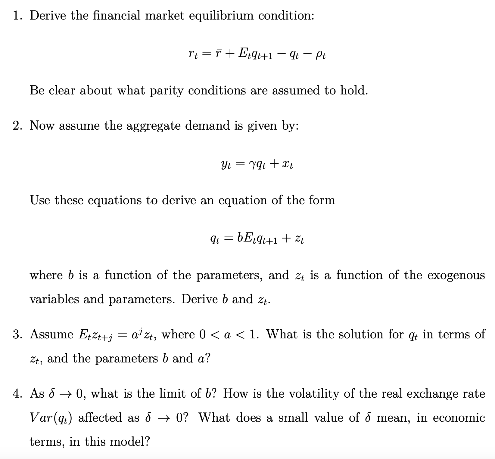
2019-P4

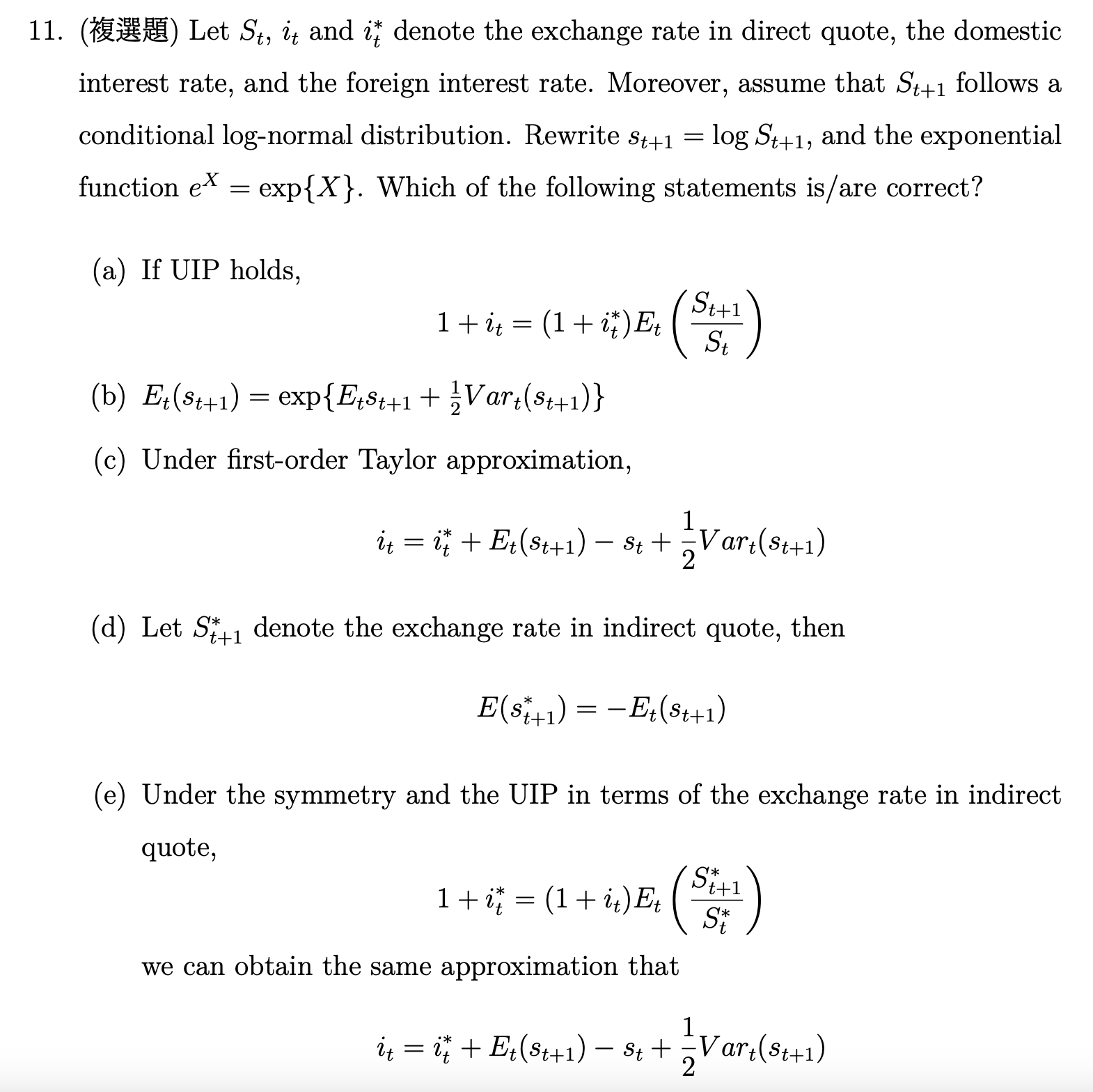
2021-P11

Ch8 Purchasing Power Parity, PPP

real exchange rate

real exchange rate \(Q_t\) = the ratio between the purchasing power of home & foreign country

\[Q_t=S_t\dfrac{P^*_t}{P_t}\]

If you can buy \(1\) big mac in the foreign country, you can \(Q_t\) big mac in the home country.

absolute PPP

weighted sum of price of a typical bundle of consumption goods

\[P=\sum w_iP_{i}\]

• purchasing power of home currency = \(\dfrac{1}{P_t}\)
• purchasing power of foreign currency = \(\dfrac{1}{P^*_t}\)
• purchasing power of home currency at foreign country = \(\dfrac{1}{S_t}\dfrac{1}{P^*_t}\)

PPP exchange rate = exchange rate to make home currency having the same purchasing power in home & foreign country

\[\dfrac{1}{P_t}=\dfrac{1}{S^{PPP}_t}\dfrac{1}{P^*_t}\]

\[S^{PPP}_t=\dfrac{P_t}{P^*_t}\]

under absolute PPP, \(S_t=S^{PPP}_t=\dfrac{P_t}{P^*_t}\)

if they're not equal, then there is opportunity for arbitrage

law of one price

a product should have the same price in a currency in every country

\[P_{it}=S_tP^*_{it}\]

This typically holds for precious metal, raw materials, luxury goods, etc., but not for general goods & services. Some reasons:

• tariffs
• international transaction cost
  • transportation cost
• long-term contracts
• pricing to market
  • some firms have some extents of monopoly power
• Principle of Macroeconomics#Sticky-Price Theory
• border effect

empirical study of absolute PPP

• it holds for developing countries with big inflations, but not for developed countries with low inflations
• in free floating regimes, the general trends follow absolute PPP

Why does it not hold

• same reasons as why #law of one price doesn't hold
• the bundle in different countries may not be the same
• the weight of the goods in the bundle in different countries may not be the same

relative PPP

there's a constant ratio between the purchasing power of two countries, which is the #real exchange rate

\[Q_t=\dfrac{S_tP^*_t}{P_t}=k\]

\[\dfrac{S_{t+1}P^*_{t+1}}{P_{t+1}}=\dfrac{S_{t}P^*_{t}}{P_{t}}\]

\[\log S_{t+1}-\log S_t=(\log P_{t+1}-\log P_t)-(\log P^*_{t+1}-\log P^*_t)=\pi_{t+1}-\pi^*_{t+1}\]

meaning the change of foreign exchange rate = the difference of inflation rate

It does not hold in short term, but does in long term.

PPP application

how much a currency is overvalued of undervalued

\[\dfrac{S_{PPP}-S}{S}\times100\]

Big Mac Index

It's good because

• big mac is a homogeneous product
• it uses local ingredient providers, reduces transportation cost
• it's sold in 120 countries