Macroeconomics
Resources
- videos
- slides and other materials
- 考古題
Ch1 intro
總體經濟學主要議題
- 長期的經濟成長
- 短期的景氣波動
- real GDP 變化以其成因
- 持續的物價膨脹
- CPI
-
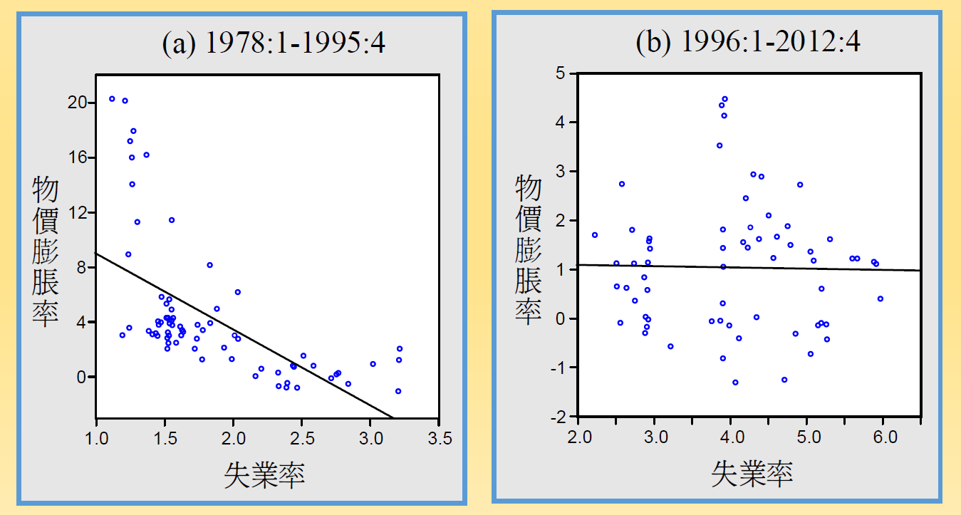
Inflation is always and everywhere a monetary phenomenon
- Milton Friedman - Philips curve
- CPI vs. unemployment rate
- 20th 兩者呈負相關
- 21st 關係不明顯
- 政府的政策干預
- 政府影響總體經濟 20th 才開始
- especially WW2 後
- transfer payment 移轉性支付
- 近幾十年來佔約 US GDP 10%
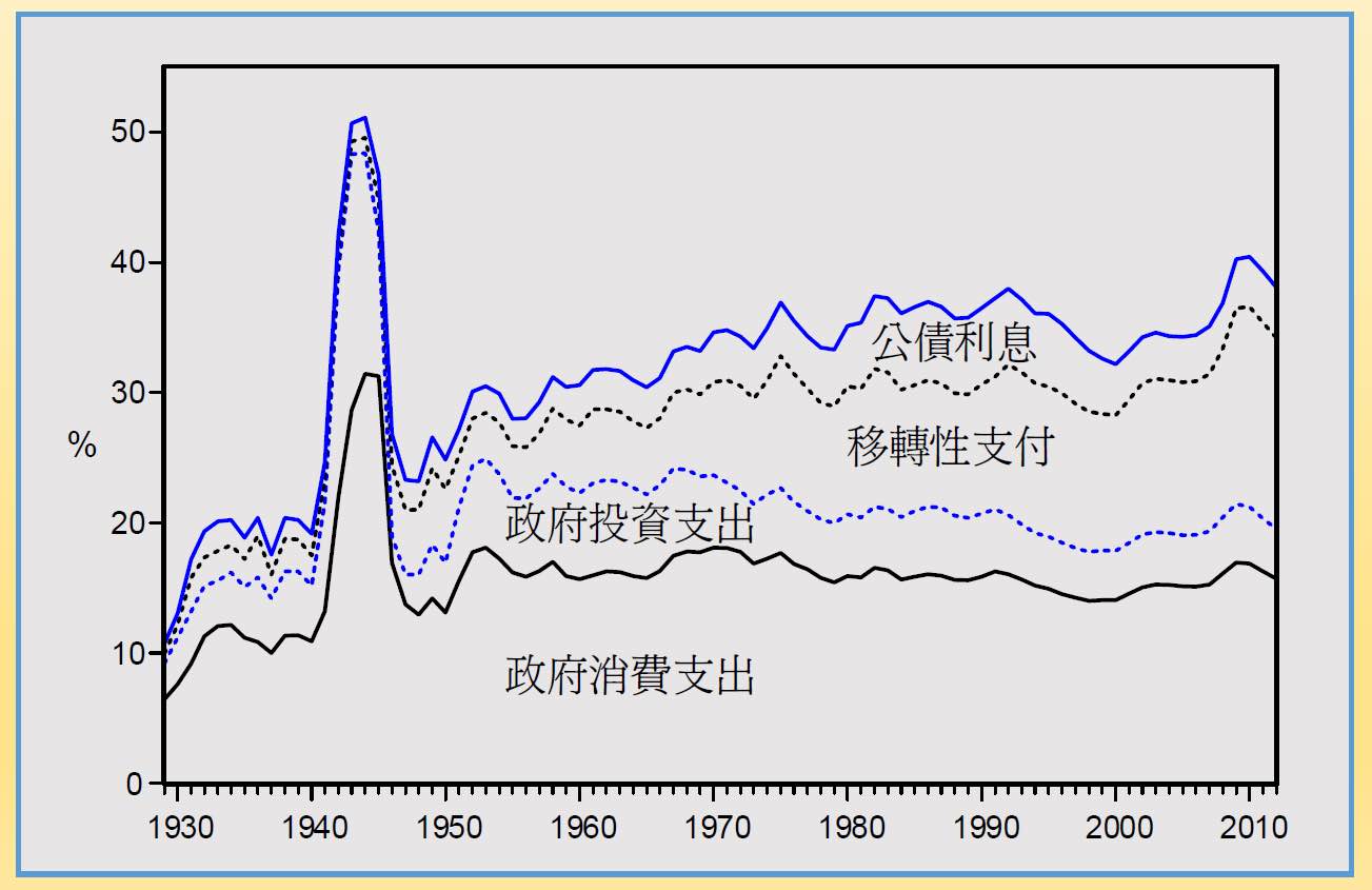
- 政府作為仲介者,左手進右手出
- e.g. 健保、消費券、社福
- 政府影響總體經濟 20th 才開始
- 金融市場的波動
- 國際貿易與金融
- US 貿易依存度
- 1970 後不斷攀升
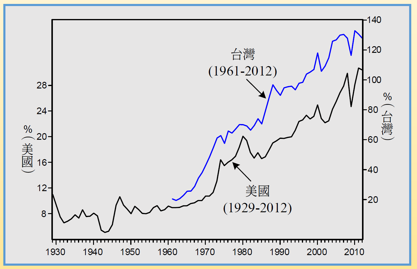
- 大部分資本移動皆為套利性質,跟貿易無關
- US 貿易依存度
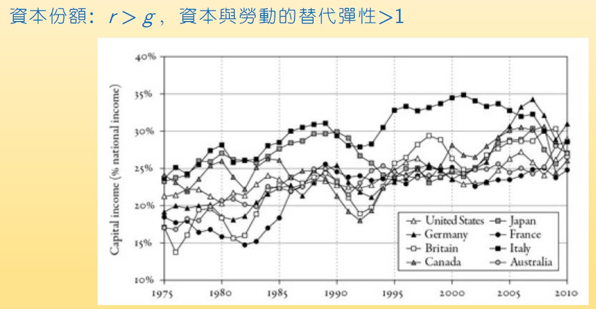
- 財富的集中與分配
- Thomas Piketty : Capital in the Twenty First Century (2014)
- 資本份額
- capital income 佔 national income 比例
- 有增加的趨勢 → 財富集中於資本家
總體理論發展史
- 古典學派 Classical School
- before 1930s
- rationality & equilibrium
- rationality: sustainable & predictable
- Say's Law 賽伊法則
- 供給會自創需求 (Keynes 對此的理解)
- 商品不會滯銷,充分就業是常態
- 無個體總體之分
- Adam Smith
- 凱因斯經濟學 The Economics of Keynes
- 1936-1950
- 1930s financial crisis
- 失業率居高不下,不符 Say's Law
- 需求自創供給
- The General Theory if Employment, Interest and Money 就業,利息與貨幣的一般理論 by Keynes
- Macroeconomics 之始
- 艱澀
- 顛覆 rationality & equilibrium
- 人類行為由 animal spirits (動物本能) 驅使
- 景氣循環沒什麼道理,不過是人類反覆的情緒
- 用 Rule of Thumb 經驗法則
- 提出很多經驗公式
- 人類行為由 animal spirits (動物本能) 驅使
- 認為他的理論較 general,不若古典理論那麼 special
- 解決 economic depression by 增加政府支出
- functional finance 功能財政
- 政府課稅、舉債 to 影響總體經濟活動
- WW2 劇增,失業的人都去從軍 → 失業問題紓解
- functional finance 功能財政
- 新古典融合 Neoclassical Synthesis
- 1950-1980
- 戰後軍費支出下降,有效需求下降,預測陷入 stagnation,US 卻反而欣欣向榮
- 因為戰爭期間民生消費品停止生產,人民沒東西買,強迫儲蓄,戰後有太多錢,消費大增,不符 Keynes 的模型
- Keynes 的消費函數的主要因素是所得,但戰後所得並無增加,只是財富增加
- 因為戰爭期間民生消費品停止生產,人民沒東西買,強迫儲蓄,戰後有太多錢,消費大增,不符 Keynes 的模型
- 凱因斯學派+理性基礎
- 統計學 & Econometrics 量化 Keynesians
- 新興古典學派 New Classical School
- 1970-
- 1974 & 1980 energy crisis,各國失業率高 & inflation rate 高,形成 stagflation (stagnation+inflation)
- 不符 Philips curve
- 各國採寬鬆貨幣政策,失業率卻沒有下降
- 不符 Philips curve
- 對 Philips curve 的批評
- Friedman
- 重要的不是 inflation rate,而是 real inflation rate 之於 expected inflation rate
- 又 inflation rate 上升時,expected inflation rate 也會上升 → expectations-augmented Philips curve 預期擴張型菲利普曲線 (see Eurozone)
- 重要的不是 inflation rate,而是 real inflation rate 之於 expected inflation rate
- Lucas
- Philips curve 會移動,斜率也會隨貨幣政策改變
- 政府想製造 unexpected Inflation → 變成垂直線 or 甚至正斜率
- Philips curve 不是 structural relationship,只是不穩定的統計相關
- Philips curve 會移動,斜率也會隨貨幣政策改變
- Friedman
- SDGE, Stochastic Dynamic General Equilibrium Model 隨機動態均衡模型
- 支持市場機制,所有市場隨時都是處於均衡狀態
- 較關心政策的長期效果
- Keynes: "In the long run, we are all dead."
- 被批為脫離現實,不知民間疾苦
- 貨幣學派、芝加哥學派
- 這堂課
- 新興凱因斯學派 New Keynesians
- 又稱新興新古典融合 New Neoclassical Synthesis
- 1995-
- new Keynesian Philips curve
- 給定 expected inflation,inflation rate & 實質產出同向移動
- 是 structural relationship 而非統計假象
- 給定 expected inflation,inflation rate & 實質產出同向移動
- 分析方法仍須用(新興)古典的方法
Ch2 產出與物價的衡量
GDP & GNI
- GDP, gross domestic product
- the market value of all final goods and services that an economy produces in a given period within its boarder
- GNI, gross national income / GNP, gross national product
- the market value of all final goods and services that an economy produces in a given period by its permanent residents
- 不是看本國籍者,而是看常住居民
- 台:半年
- 不是看本國籍者,而是看常住居民
- the market value of all final goods and services that an economy produces in a given period by its permanent residents
- final output 附加價值/最終產出/生產價值
- 生產總值 - 中間投入
- 差異:生產要素 (labor & capital) 的跨國移動
- GNI/GNP = GDP + NFIA
- NFIA, net factor income from abroad
- 國外要素所得 - 國外要素支出
- 國外要素所得
- 去國外賺的錢
- {residents outside of broader}'s income
- 國外要素支出
- 給外來人的錢
- {non-residents within broader}'s income
- e.g. 外勞薪資
- 國外要素所得
- 國外要素所得 - 國外要素支出
- flow variable 流量變數
- in a range of time
- GDP & GNI
- stock variable 存量變數
- at a specific time
- 機器設備、存貨、餘額
- 僅涵蓋有市場交易的 goods and services
- 地下經濟、主婦勞務不算
- 政府活動以政府決算支出&生產成本為計價基礎
- 國防司法外交治安
GDP 的三個面向
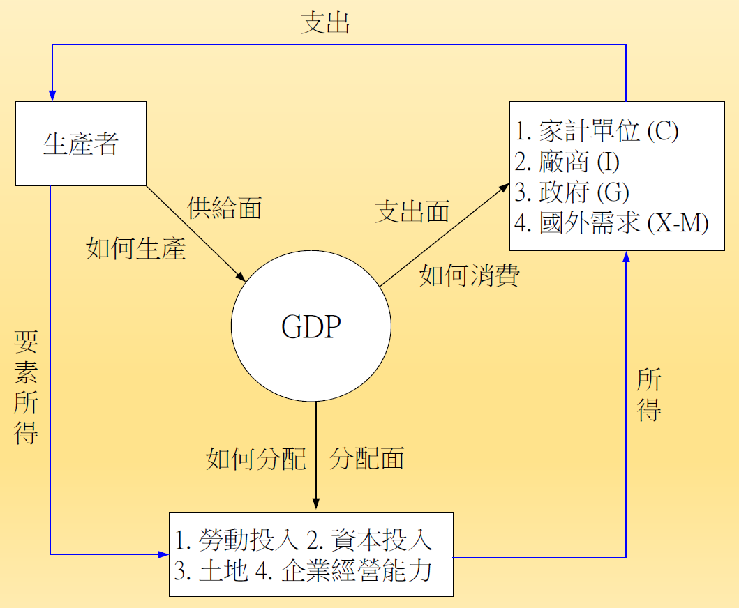
- 供給面
- 生產者
- 支出面
- 誰吃掉?
- 家計單位
- 廠商
- 政府
- 國外需求
- 誰吃掉?
- 分配面
- 生產要素
- 勞動
- 資本
- 土地
- 企業經營能力
- 生產要素
- 供給面
- 三個面的計算結果會一致
生產面
- 用聯合國會計準則 SNA08
- GDP = 境內所有生產者創造的生產價值
- 生產價值 / 最終產出 = 生產總值 - 中間投入
- 中間投入 = 投資支出-無形投資
- 投資支出
- 可能在未來創造利潤的支出
- 無形投資沿革
- SNA93 新增企業軟體支出 & 礦藏探勘費用 → 不算在中間投入
- SNA08 新增廠商研究發展(R&D) & 專利權支出 → 不算在中間投入
- 存料不算中間投入,so 買 20 顆 CPU 生產&賣掉 10 台電腦,中間投入只要減掉 10 顆 CPU 的價格
- 投資支出
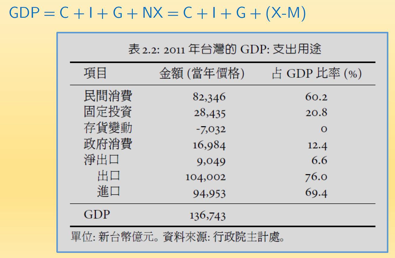
支出面
- Y = domestic output = GDP
- C = Consumption = 民間消費支出
- 占比最高,60-70%
- 波動不大
- 依消費屬性
- nondurables 非耐久財消費
- 2011 佔台 24%
- 實體商品
- durables 耐久財消費
- 2011 佔台 24%
- 包括主計處的半耐久財消費
- services 服務消費
- 2011 佔台 52%
- 包括自有住宅的設算租金
- 估計自有住宅創造的價值
- nondurables 非耐久財消費
- I = Investment = 國內投資支出/固定資本形成毛額
- 生產者購買資本財的支出
- 約 20%
- 波動幅度大
- 依所有主
- 民間投資
- 2011 佔台 15.8%
- 公部門投資
- 2011 佔台 5%
- 政府投資
- 公營企業投資
- 民間投資
- 依資本財屬性
- 實體投資/有形投資
- 2011 佔台國內投資 93%
- 無形投資
- 企業 copyright fee
- SNA93 納入企業軟體支出、礦藏探勘費用
- SNA08 納入研究發展 & 專利權支出
- 存貨變動 Inventory accumulations
- 期末 - 期初存貨
- flow variable
- 今年生產但沒有賣掉 → 存貨增加
- 實體投資/有形投資
- DEP, depreciation
- 資本耗損/折舊
- net investment = gross investment - depreciation
- NDP = GDP - DEP
- net domestic product
- NNI = GNI - DEP - net national income
- 期末資本存量 = 期初資本存量 + 淨投資
- G = Goverment purchases = 政府消費支出
- 以實際決算為計價基礎
- 有些並未透過市場完成
- 2011 佔台 12.4%
- 偏低
- 政府預算支出
- 消費性支出
- 投資性支出
- exclude transfer payments
- 公債利息
- social welfare benefits
- 以實際決算為計價基礎
- NX = Net Exports = X - M = 淨出口/ trade surplus 貿易盈餘
- merchanting trade 三角貿易
- e.g. 鴻海台灣資,中國生產,美國買 (iphone)
- 以銷貨淨額 (output-input) 計入 GDP
- X
- 出口
- M
- 進口
- merchanting trade 三角貿易
分配面/要素所得面
- 國民所得 National Income (NI)
- = 工資 + ( 利息 + 地租 + 利潤 )
- 利息包含地租以外的租金
- 店租、房租、資本租金 etc.
- 利潤是減掉 NIT (間接稅淨額) & DEP (折舊) 後
- 間接稅淨額 Net Indirect Tax (NIT) = 間接稅 - 生產補貼
- 間接稅
- 營業加值稅
- 關稅
- 生產補貼
- 出口補貼
- 雜糧補貼
- 不勞而獲
- 間接稅
- 間接稅淨額 Net Indirect Tax (NIT) = 間接稅 - 生產補貼
- GDP = DI + ( DEP + NIT )
- GNI = NI + ( DEP + NIT )
- 把減項加回來
- 利息包含地租以外的租金
- = 受僱人員報酬 + 營業盈餘 (混合所得)
- 屬籍
- = 國內要素所得 Domestic Factor Income (DI) + NFIA
- = 工資 + ( 利息 + 地租 + 利潤 )
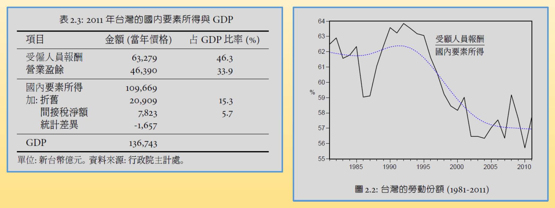
- 受僱人員拿到的份變少
real GDP
- nominal GDP / GDP at current price != real output
- 需減掉價格波動
固定價格 GDP (GDP at constant prices)
- 選擇一個固定的 base period,以基期價格計算各期 GDP
- 不同的 base period 選擇會有不同的成長率
- 忽略了商品間相對價格的變動
- 需要定期改變基期
連鎖加權 GDP (chain-weighting GDP)
- Fisher Quantity Index \(F^Q_t\)
- 實質產出成長率
- 以兩個基期計算的 GDP 成長率的幾何平均數
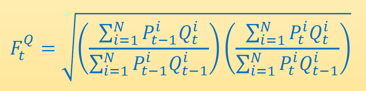
- \(F_t^Q=\sqrt{(1+g_t^1)(1+g_t^2)}=1+\bar{g_t}\)
- \(\bar{g_t}\) = 費雪成長率
- chained index
- GDP 複率成長
- \(I_t=I_{t-1}\times F^Q_t= ...=F^Q_1\times F^Q_2\times ...\times F^Q_t\)
- chain-weighting GDP
- \(Y^C_t=I_t\times Y_0=(F^Q_1\times F^Q_2\times ...\times F^Q_t)\times Y_0\)
- \(Y_0\) = base period nominal GDP
- e.g.
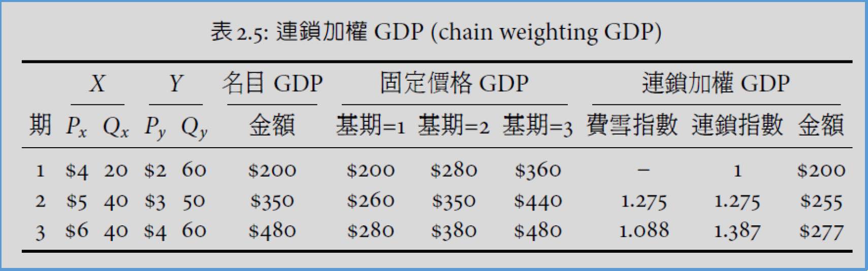
- ((260/200)x(350/280))^0.5=1.275
- 200x1.275=255
- ((38/35)x(48/44))^0.5=1.088
- 1.275x1.088=1.387
- 200x1.387=277
- pros
- 較能反映鄰近期間實際生產活動變化
- cons
- 非線性轉換 → GDP=C+I+G+NX 不成立
購買力平價 GDP (purchasing power parity GDP)
- PPP-GDP
- 以基準商品籃建立國際貨幣單位 international dollar
國民所得&國民儲蓄
民間儲蓄 private saving
- 家計所得 household income
= 要素所得 + 政府移轉所得 (TR) + 公債利息 (INT, interest income) - 廠商盈餘
= GNI - 要素成本
= (GDP + NFIA) - 要素成本- 生產者附加價值 = GNI
- 民間所得 private income
= 家計所得 + 廠商盈餘
= GNI + TR + INT
= GDP + NFIA + TR + INT - 民間可支配所得 private disposable income
\(Y^P\)= (家計所得 + 廠商盈餘) - TAX (直接稅 + 間接稅淨額)
= (GDP + NFIA + TR + INT) - TAX- TAX
- 家計單位繳直接稅
- 廠商繳間接稅淨額
- TAX
- 民間儲蓄
\(S^P\) = 民間可支配所得 (\(Y^P\)) - 民間消費支出 (C)
= (GDP + NFIA + TR + INT) - TAX - C
政府儲蓄 government saving
- also knows as public saving
- 政府儲蓄
\(S^G\) = TAX - (G + TR + INT)
= 政府投資支出 + 政府預算盈餘
= 政府投資支出 - 政府預算赤字- 政府預算盈餘 budget surplus = 總稅收 - 總支出
= TAX - (G + TR + INT + 政府投資支出) - TAX 包含公營事業盈餘等
- 政府預算盈餘 budget surplus = 總稅收 - 總支出
國民儲蓄 national saving
- S (國民儲蓄) = \(S^P\) (民間儲蓄) + \(S^G\) (政府儲蓄)
= GNI (國民所得毛額) - ( C (民間消費) + G (政府消費) )
= (GDP + NFIA) - (C + G)
= (C + I + G + NX + NFIA) - (C + G)
= I + (NX + NFIA)
= I (國內投資支出) + CA (經常帳盈餘) - 國民儲蓄 - 折舊
= 國民儲蓄毛額 gross national saving - 折舊
= 國民儲蓄淨額 net national saving - 經常帳盈餘 (CA, current account) = 貿易盈餘 (NX) + 國外要素所得淨額 (NFIA)
- 國外資產持有 = 對外國住民的求償權
- CA > 0 → 國外資產淨額增加 i.e. 對外國住民求償權增加,資本帳赤字
- current account + 資本帳 (capital account) = 0
- 國民儲蓄 S = I + CA 流向
- 留在國內 → 國內投資支出 (I)
- 若也沒有做有形 or 無形投資,則只會讓存貨增加
- Keynesian: paradox ot thrift
- 儲蓄是一種罪惡,會使均衡產出下降
- 你 save → 別人的 income 減少 → overall saving drop in the long term
- Keynesian: paradox ot thrift
- 若也沒有做有形 or 無形投資,則只會讓存貨增加
- 流向國外 → 經常帳盈餘 (CA) i.e. 以商品或要素形式流向國外
- e.g. 買 US treasury OR 國外資產 (???????????????? 到底是金錢還是商品或要素形式流出)
- CA > 0 → 國民儲蓄 → 國內投資 → 超額儲蓄 excessive saving
- 代表賺來的錢沒被消費掉
- 期末資本存量 = 期初資本存量 + 淨投資 (I)
- 期末國外資產淨額 = 期初國外資產淨額 + 經常帳盈餘 (CA)
- 留在國內 → 國內投資支出 (I)
物價指數 price index, general price level
GDP 平減指數 (GDP Deflator)
- GDP Deflator = nominal GDP / 固定價格 GDP x 100
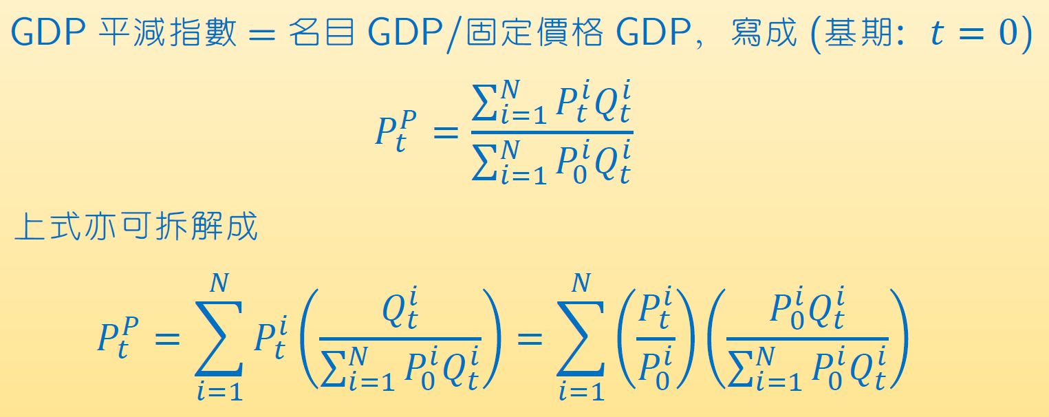
- base period: 0
- 利用當期支出比重做加權平均
- sum{ i 商品漲價幅度 x 佔 GDP 的比例} i.e. 商品漲價幅度加權平均
- intuition: 現在的商品拿去過去賣,漲了多少
- 分母:現在的商品數量用過去的價格算
- Paasche index, 使用當期消費量
- 會低估 inflation
- a 商品長特別凶 → 均衡數量降低 → a 商品加權較少 (substitution effect)
- 無法排除商品相對價格的影響
- 會低估 inflation
消費者物價指數 (CPI, consumer price index)
- 用 retail price
- 生產者物價指數 WPI 用 wholesale price
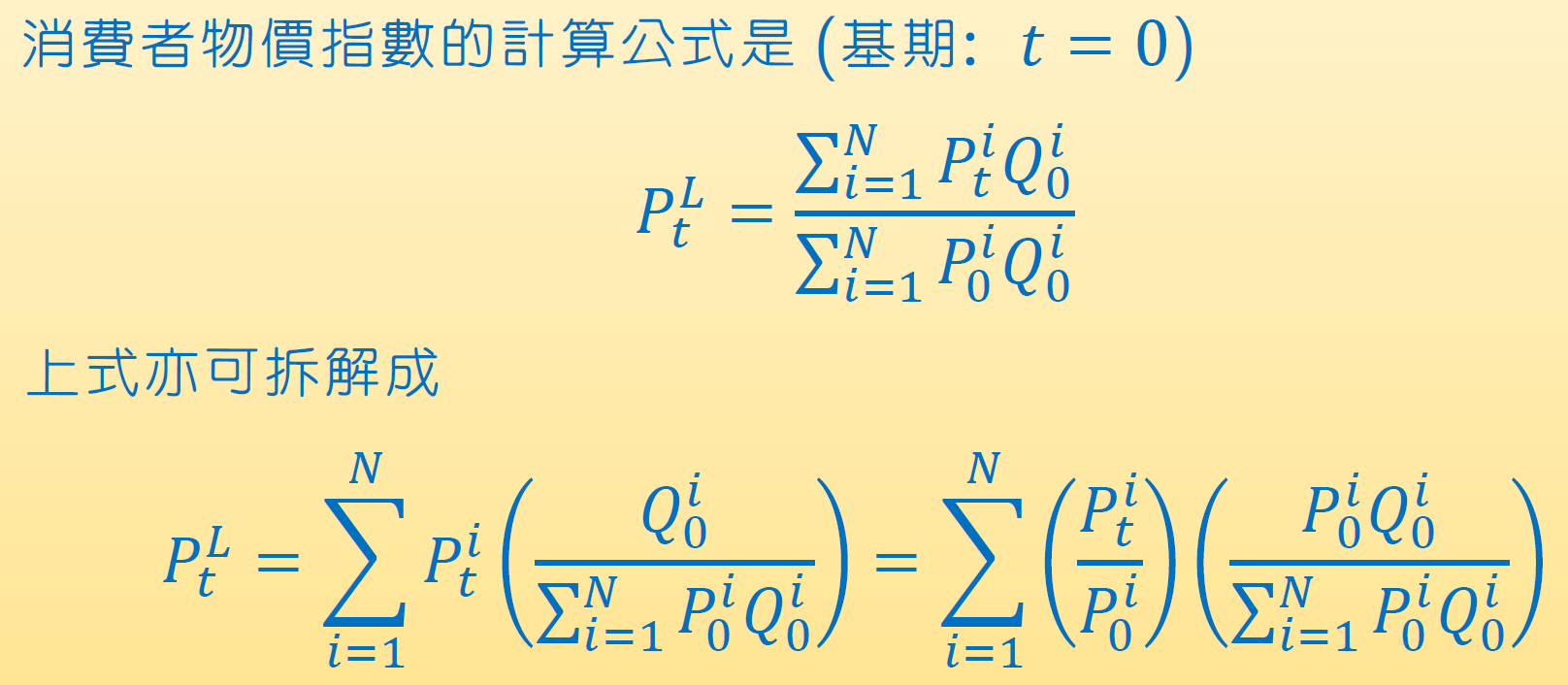
- base period: 0
- intuition: 過去的商品拿來現在賣,貴了多少
- 分子:過去的商品數量用現在的價格算
- 利用基期支出比重做加權平均
- Laspeyres index, 使用 base period 消費量 i.e. 價格改變前的消費量
- 會高估 inflation
- 忽略人們會少買漲得多的東西 (substitution effect)
- 會高估 inflation
PCE deflator, personal consumption expenditures deflator
- Fisher Price Index \(F^P_t\)
- 物價上漲率
- like Fisher Quantity Index \(F^Q_t\) but 變動項為 price
- 現在的數量拿去過去 (Paasche) & 過去的數量拿來現在 (Laspeyres) 的幾何平均
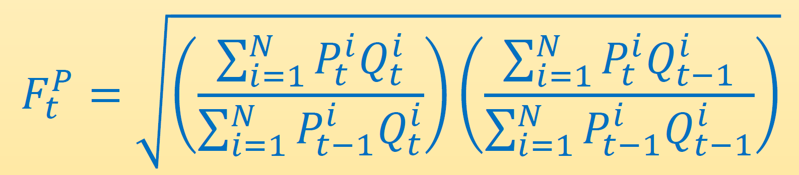
- \(F^P_t\times F^Q_t=\dfrac{Y_t}{Y_{t-1}}\)
i.e.物價上漲率 x 實質產出成長率 = 名目 GDP 成長率
- \(P^C_t=F^P_1\times F^P_2\times...\times F^P_t\)
- \(P^C_t\times Y^C_t=Y_t\)
i.e.物價指數 x 實質 GDP = 名目 GDP - 介於 Paasche & Laspeyres 之間,考慮了相對價格的影響 → 較能反映 inflation
- 使用滾動基期 → 較能反映貨幣政策對物價的實際影響
- Fed 政策主要參考指標
e.g.
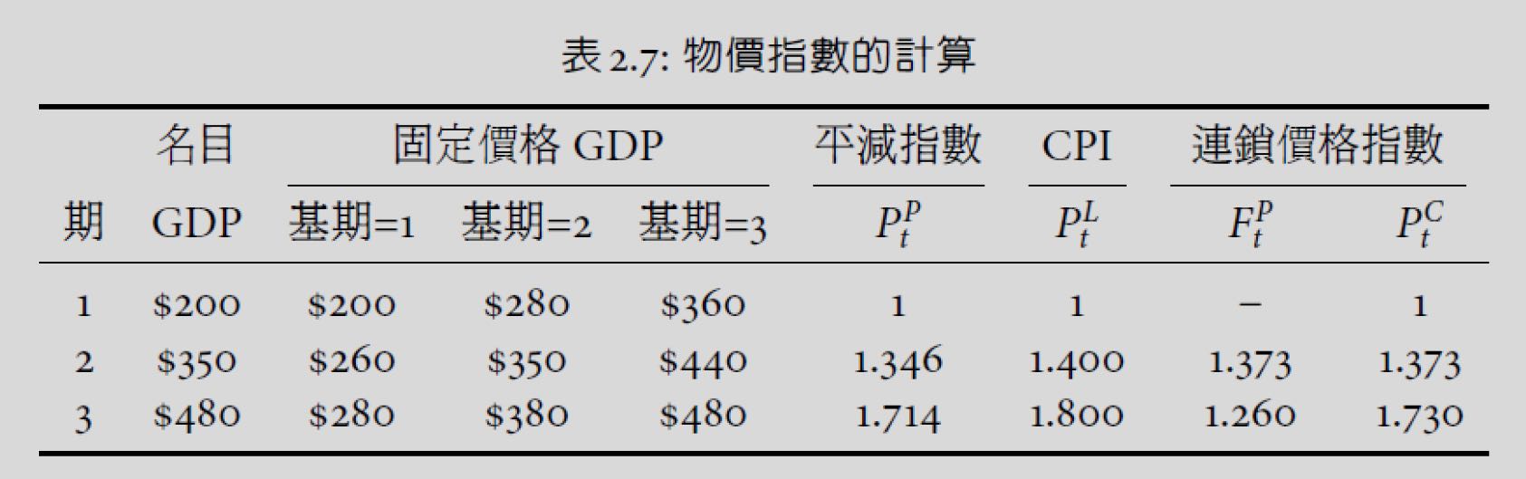
- 350/260 = 1.346
- 280/200 = 1.400
- (1.3461.4)*0.5 = 1.373
- ((440/350)(480/380))*0.5 = 1.260
- 1.373*1.260 = 1.730
Problems
Ch3 景氣波動的定型特徵
- business cycle 景氣循環
- real GDP 隨著長期趨勢上下波動的 stochastic process
filtering
- 把短期波動獨立濾出來
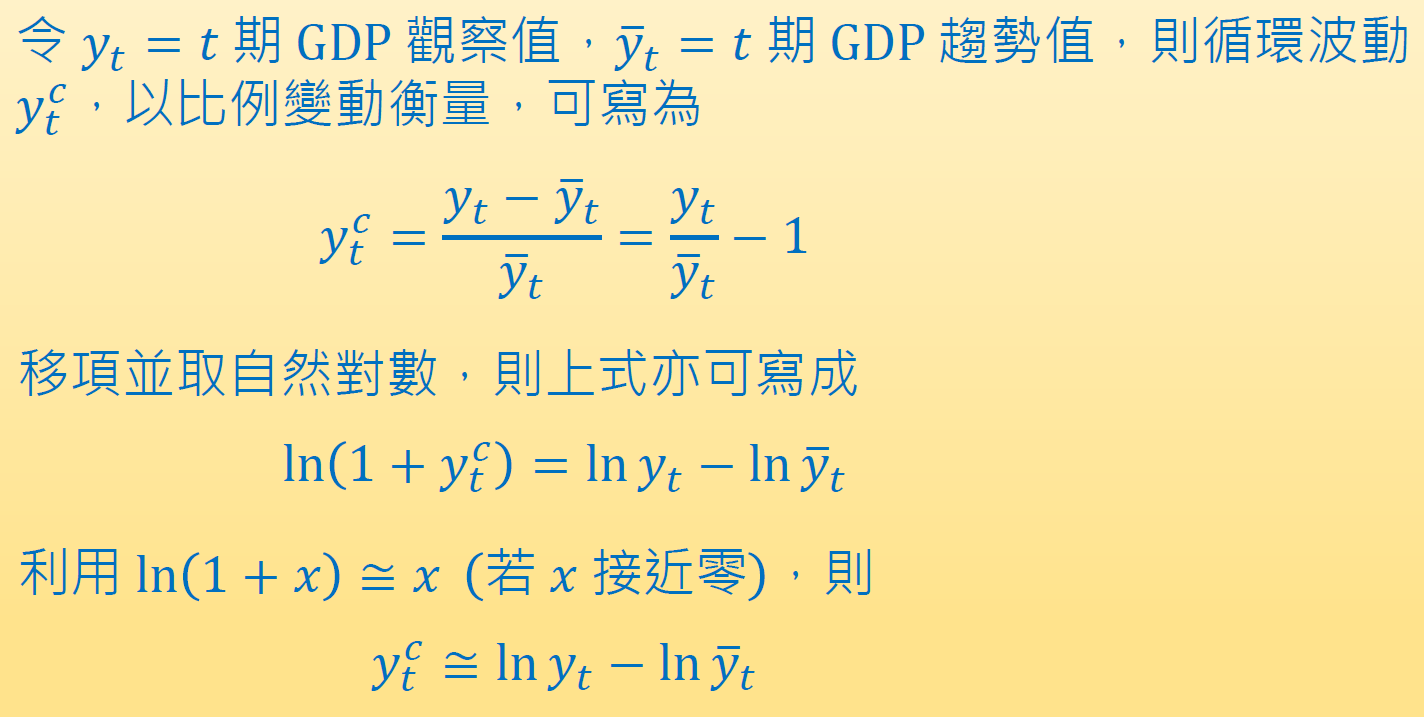
- 各期產出 = 長期趨勢 + 短期波動
- 波動比例 = 實際&趨勢差異 / 趨勢值
產出成長率濾波器
- 產出成長率 = \(\dfrac{y_t-y_{t-1}}{y_t}=\ln y_t-\ln y_{t-1}\)
- \(\ln y_t\) vs. t 圖之斜率 = 產出成長率
- \(\ln y_t\) vs. t 圖之斜率 = 產出成長率
- 將上一期視為長期趨勢值
- 顯然不合理
- 長期趨勢太波動
- 可能濾掉很多短期波動 → over differencing
- 顯然不合理
- 寫成時間的線性函數
\(\ln \bar{y_t}=\alpha+\beta t\),留下跟時間無關的 \(\alpha\)- 直接假設長期波動 not a function of 時間 → 不合理
- 長期趨勢太淡定
- \(\alpha\) 可能包含了長期波動 → under differencing
- 直接假設長期波動 not a function of 時間 → 不合理
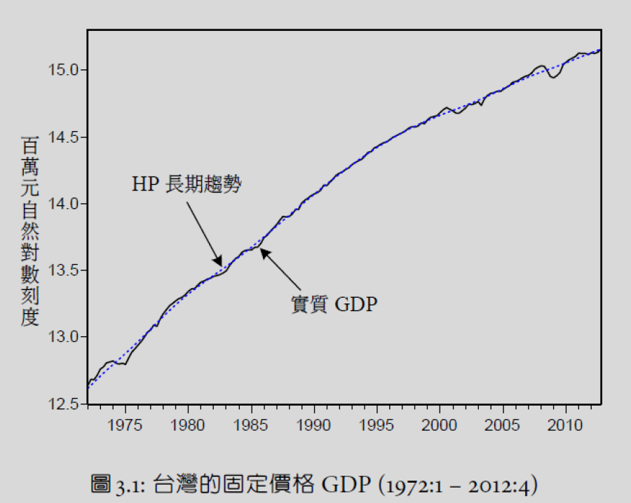
HP 濾波器
- Hodrick-Perscott filter
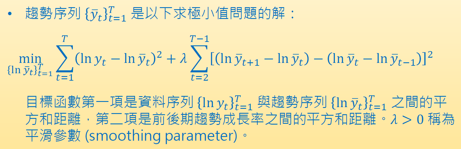
- 只有第一項 → 長期&實際愈接近愈好
- 只有第二項 → 長期愈 linear 愈好
- \(\lambda\) 平滑參數控制第二項的 weight
- \(\lambda=1600\) for 季資料
- \(\lambda=100\) for 年資料
- HP 循環波動序列 = \(\ln y_t-\ln \bar{y_t}\)
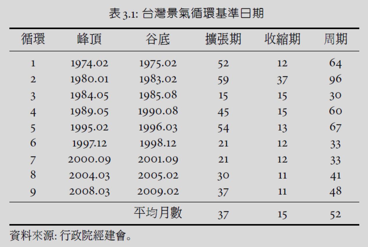
- 台以 HP 循環波動序列做景氣轉折點的認定
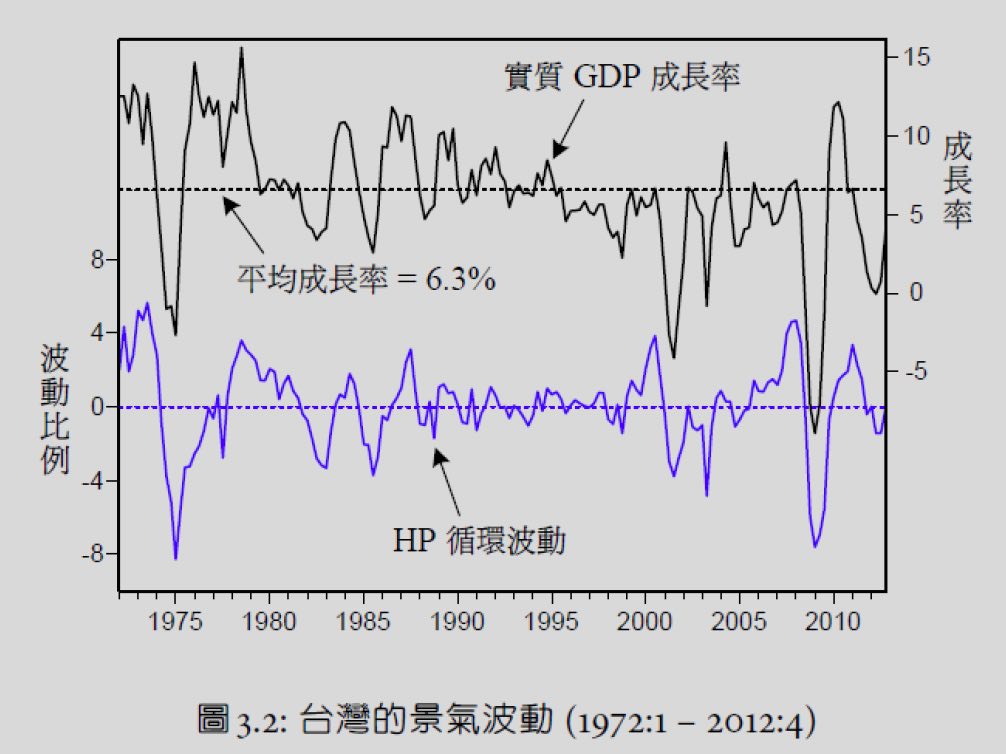
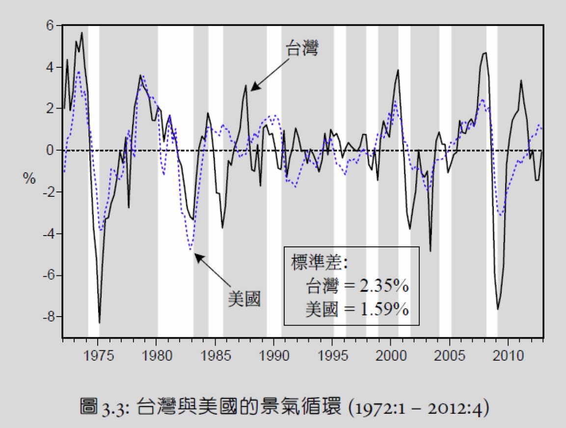
台美景氣波動
- 台美景氣波動很接近
- 1972-2012 台經歷 9 次景氣循環
- 景氣循環都是跌得快漲得慢
- 睡眠週期的相反
- 台 std 較美大 bc 台灣較小,應對衝擊能力較低
- 約 2-6 年一次 cycle
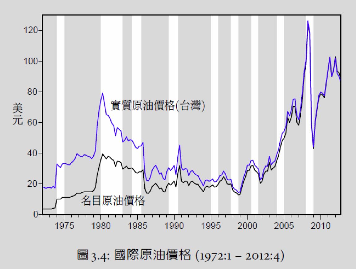
第一次能源危機
- 1973 以阿戰爭,阿拉伯向西方實施石油禁運,國際油價大漲
- 停滯性膨脹
第二次能源危機
- 1979 Iran 回教革命,1980 兩伊戰爭,原油供給受干擾,油價大漲
廣場協議
- 1985 要求日德幣升值
- 新台幣也受牽連升值,出口導向的台灣陷入衰退
第三次能源危機
- #廣場協議後,預期新台幣升值 → 國際熱錢湧入台灣 → 股市蓬勃
- 1990 Iraq 入侵科威特,波斯灣戰爭爆發 → 熱錢流出、預期油價上漲 → 股市崩跌
台海飛彈危機
- 1995-1996 小幅度衰退
- NBER 未認定有景氣衰退
亞洲金融風暴
- 1997 泰國放棄固定匯率,George Sorus 等炒家突襲外匯市場,泰銖暴跌,一路往北跌到俄羅斯
- 台灣替手新台幣,讓炒家過門不入,因此受創就輕微 ???
- 經濟衰退 → 原油需求下降 → 國際油價下跌
dot-com bubble
- 20th 末
- 同時台灣 1999 921、2000 政黨輪替 & 美國 911
- 經濟衰退 → 原油需求下降 → 國際油價下跌
次貸危機
- 2007 年底
- #dot-com bubble 後,US 採寬鬆貨幣政策 → 房價大漲 → 高槓桿金融商品
- 包很多層的避險衍生性商品
- 2010-11 歐債危機
- US 因 QE 沒受什麼影響
- 也對國際油價沒什麼影響
景氣波動 3 面向
波動幅度 volatility
- 經過處理的標準差

- 分母應是 T-1 但沒什麼差
- 處理過後再計算標準差才有意義
- 原始資料包含長期趨勢的影響,為 non-stationary 時間序列,因此要先用 #filtering 濾成 stationary 序列
- 可證明 HP 循環波動必為 stationary
- s.t. 標準差是相對於長期趨勢的標準差 i.e. 在長期趨勢上下波動的幅度
- 原始資料包含長期趨勢的影響,為 non-stationary 時間序列,因此要先用 #filtering 濾成 stationary 序列
變數同步性 co-movement
- 順循環 pro-cyclical
- x y covariance > 0
- 逆循環 counter-cyclical
- x y covariance < 0
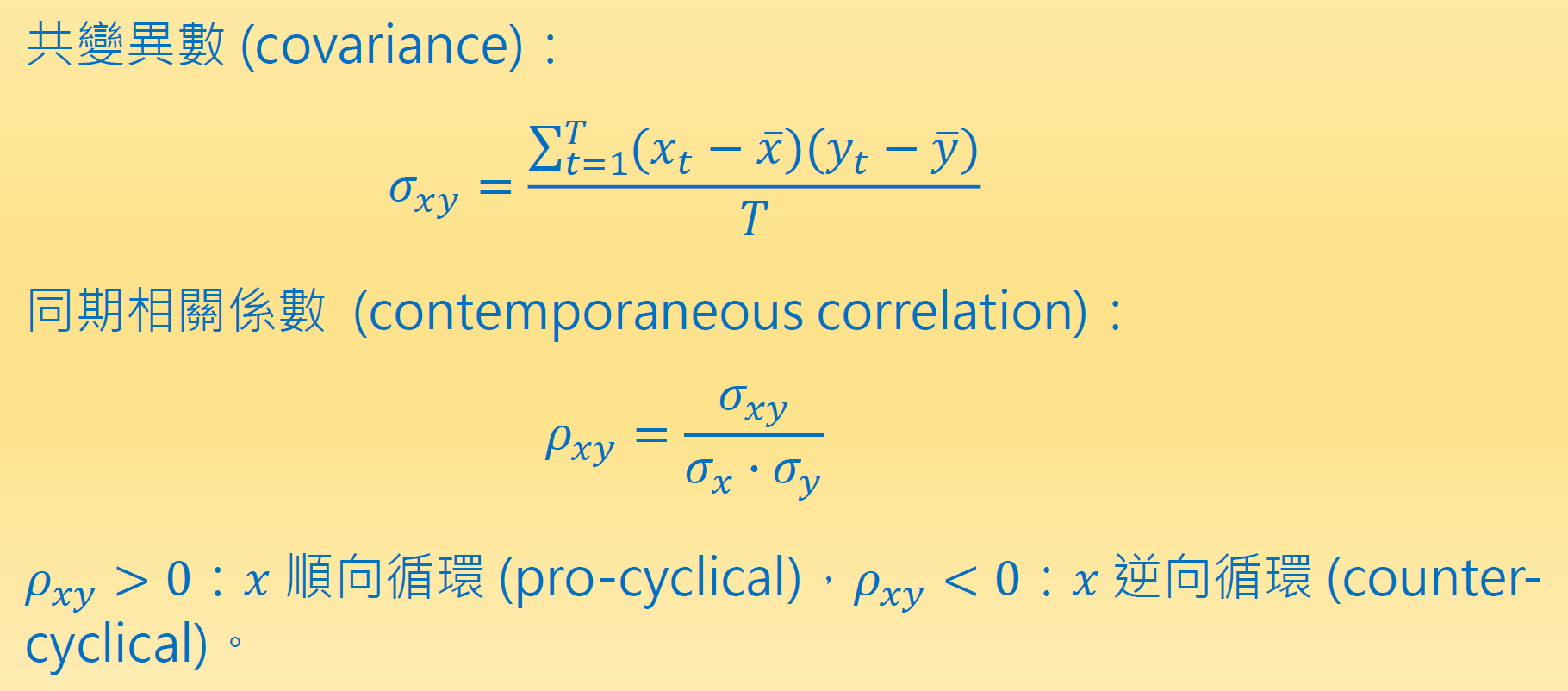
- covariance 大小不代表相關強度,bc 受 x or y 單位 or 標準差影響
- correlation \(\centernot{\implies}\) causation
- 相關係數只說明了 x y 間的線性關係,無法說明非線性關係
- e.g. y=|x| 相關係數 = 0 但顯然有關係
波動持續性 persistence
- 跨期相關
- auto-covariance 自我共變異數
- 當期跟 j 期以前的 covariance
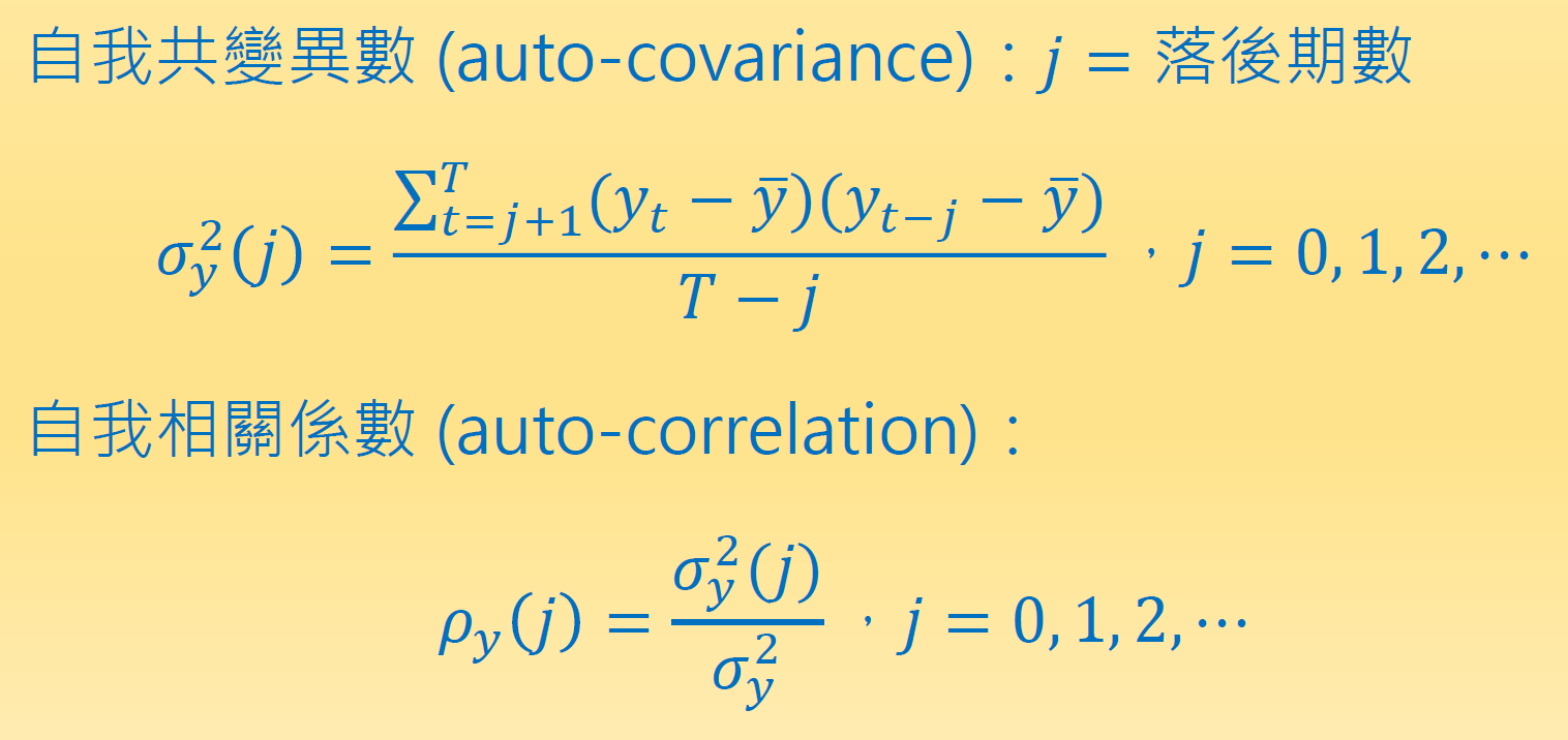
- 隨著 j 增加而遞減 (intuitive)
- cross auto-covariance
- x 跟 j 期外的 y 的 covariance
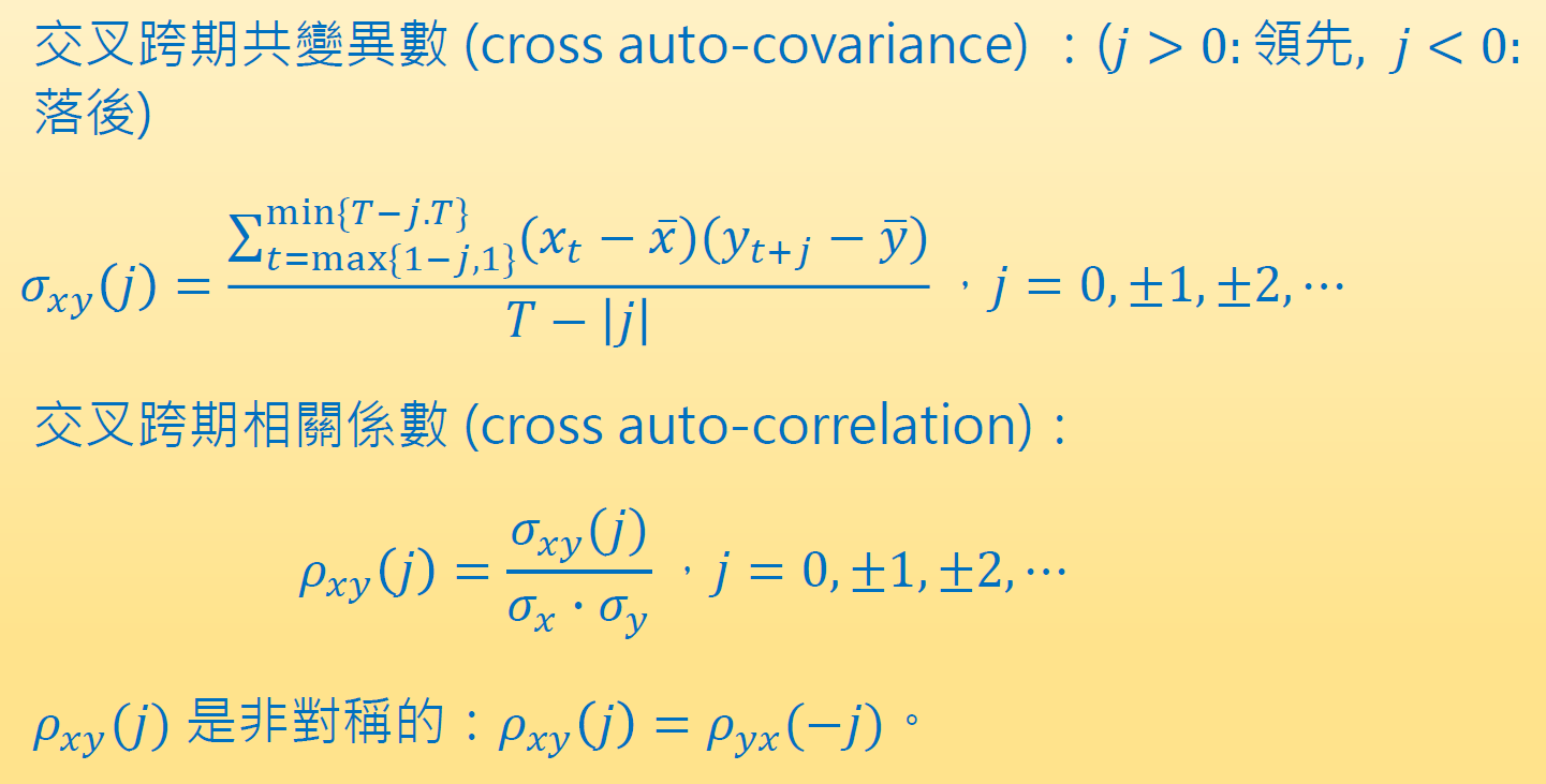
- j > 0 → 領先期
- j < 0 → 落後期
- \(p_{xy}(-1)>0\) → 今天消費與昨天所得呈正相關
- 不能用於判斷因果關係
- Granger causality test
台美氣波動定型特徵
- 實質利率
- 台:一個月平均款利率
- 美:三個月國庫券利率
- 實質利率
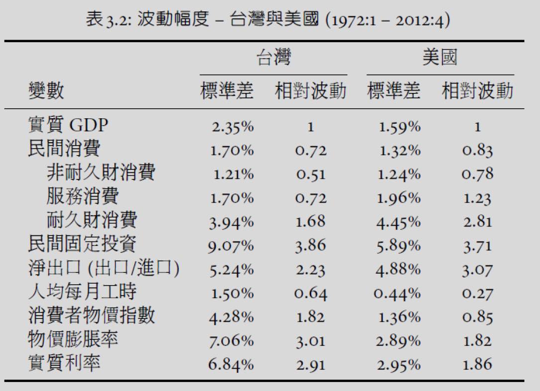
波動幅度
- smooth consumption
- 民間消費波動幅度 < 實質產出波動幅度
- 凱因斯學派解釋
- \(c=a+by\) \((a>0 \implies c>by)\)
- \(\dfrac{c-\bar{c}}{\bar{c}}=b\dfrac{\bar{y}}{\bar{c}}\dfrac{y-\bar{y}}{\bar{y}}<\dfrac{y-\bar{y}}{\bar{y}}\)
- 新興古典學派解釋
- 景氣繁榮 → save 部分額外所得 i.e. 增加儲蓄
- 景氣衰退 → 減少儲蓄
- 耐久財波動幅大較大
- bc 較貴,景氣衰退時更不買,景氣繁榮時更買
- 民間固定投資波動幅度 > 實質產出波動幅度
- 景氣衰退時減少資本財購買 (just as 耐久財)
- 景氣繁榮 → #國民儲蓄 national saving 上升 → 資本存量增加 if 流向國內投資
- 與 smooth consumption 為一體兩面
- 凱因斯學派解釋:multiplier-accelerator model
- 貿易盈餘波動幅度 > 實質產出波動幅度
- 景氣繁榮 → #國民儲蓄 national saving 上升 → 經常帳盈餘增加 if 流向國外
- 勞動工時波動幅度 < 實質產出波動幅度
- 勞動窖藏 labor hoarding
- hire & fire 勞工有成本&風險
- 不景氣 → 就讓勞工閒著
- 景氣 → 狠操勞工
- leisure 也是一種 consumption
- 勞動窖藏 labor hoarding
- inflation rate & real interest rate 波動幅度 > 實質產出波動幅度
- real interest rate = 消費&投資的機會成本
- 美國是相反
- 台灣前兩次能源危機物價波動太激烈
- 除去前兩次能源危機後,也是小於
同期相關
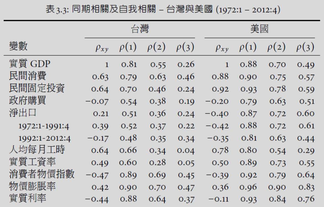
- 民間消費&民間投資是順循環
- 跟 real GDP 一起浮動
- 政府購買&產出波動無明顯同期相關
- 不代表政府支出政策對產出沒影響,可能只是個因素互相抵銷
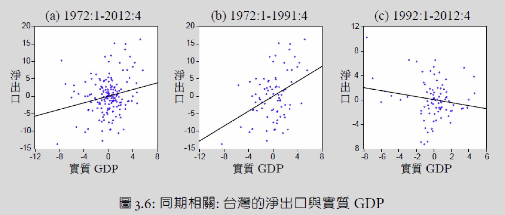
- 台淨出口&產出波動正相關,美負相關
- 景氣繁榮時出口增加 > 進口增加 for 台灣 (before 1992),相反 for US&others
- 1992 後台灣也是負相關
- 勞動工時&實質工資率為順循環
- 物價水準與 real GDP 逆循環
- 相對於長期趨勢,景氣繁榮時物價較低
- inflation rate 與 real GDP 順循環
- 又 unemployment rate 與 real GDP 負相關 → inflation rate 與 unemployment rate 負相關 → Philips curve
- real interest rate 與產出波動負相關
跨期相關
- 高度跨期自我相關
- 傳導機制 propagation mechanism
- smooth consumption & 資本累積
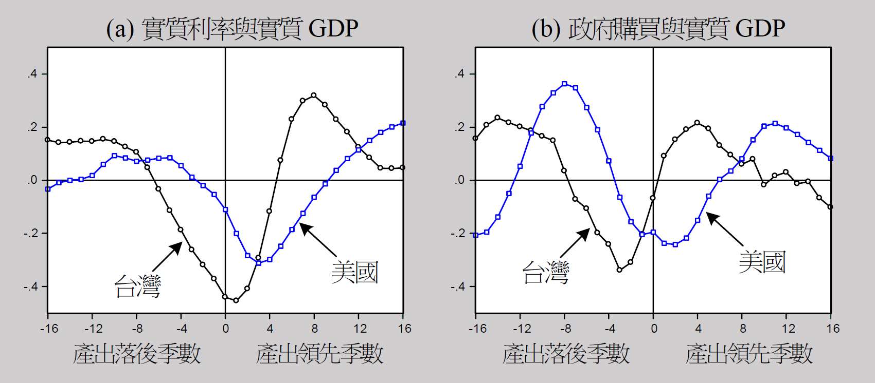
- 台 real interest rate 跟前後一年 real GDP 負相關
- US real interest rate 跟未來一年 real GDP 負相關
- 台政府支出與過去一年 real GDP 負相關,與未來一年 real GDP 正相關
- 景氣衰退時採取寬鬆貨幣政策,一年後效果顯現
- 美政府支出與未來一年 real GDP 負相關,與兩年後 real GDP 正相關
Ch4 廠商的靜態選擇
no tomorrow in static model
- no savings
- no investment
模型
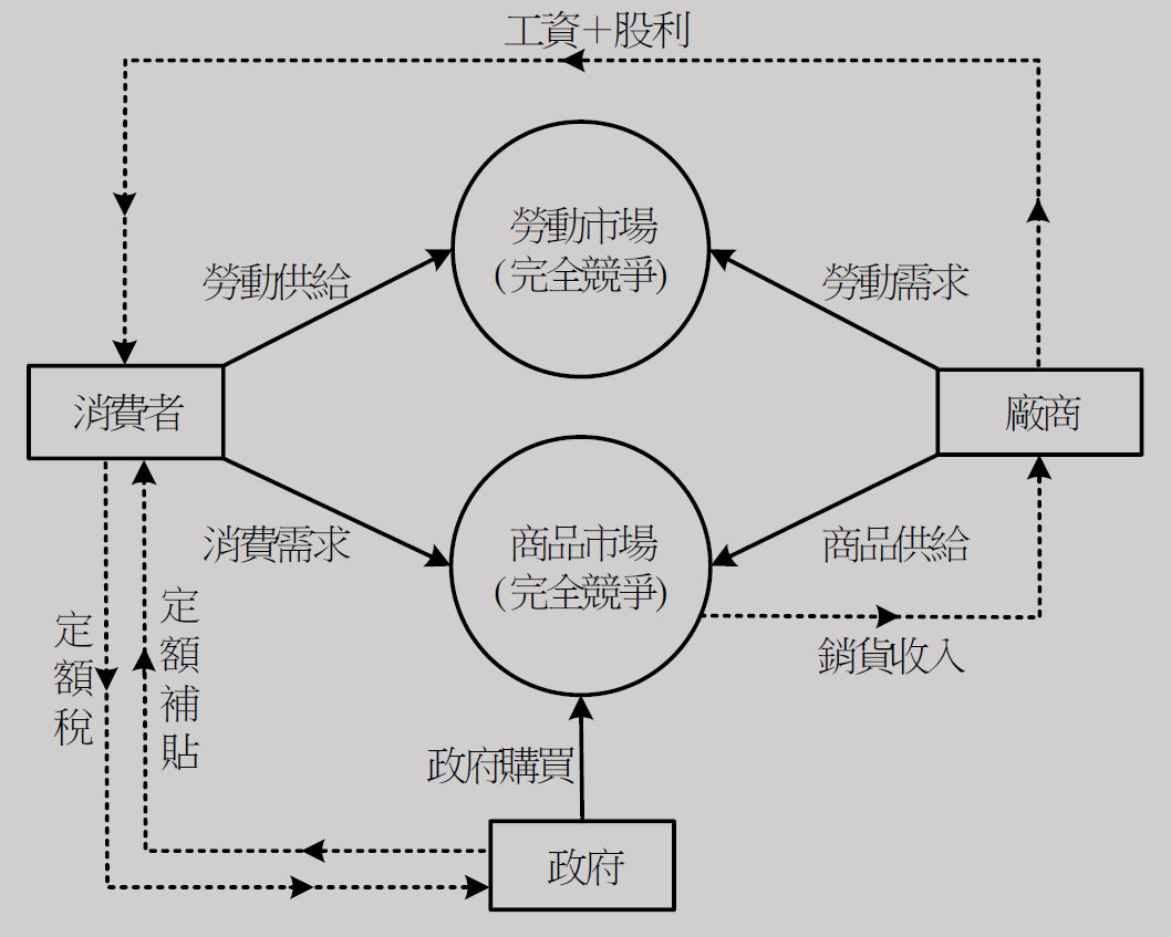
labor market & goods market are in perfect competition
- consumer & firm 都是 price taker
- 廠商生產 homogeneous products
角色
- 廠商
- 收入
- 付工資
- 以股利分給消費者
- 屬於消費者
- so 不用繳稅
- 收入
- 消費者
- 繳稅
- 定額稅淨額 net lump-sum tax = 定額稅 - transfer payment
- 定額 lump-sum
- 大家都繳一樣的
- 可支配所得 = 工資+股利-定額稅淨額
- 全部用於消費
- 繳稅
- 政府
- 收入
- 課定額稅 from 消費者
- 支出
- transfer payment
- 買商品
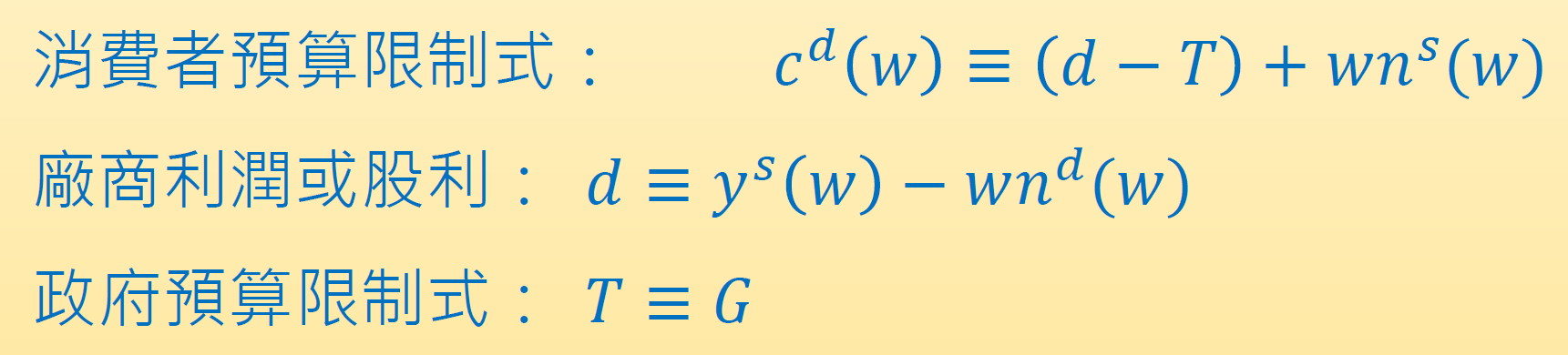
- 課稅量 = 支出
- no 借貸 no 公債
- 收入
特性
- barter economy
- 沒有貨幣
- 以商品為計價單位 (numeraire)
- 實質工資率
- 無 nominal
- closed economy
- 無貿易
生產函數
- 代表性個人模型 representative agent model
- 所有單位都一樣
- y = 產出
- k = capital
- n = labor
- A, B = 生產面衝擊
- 影響生產的東西
- A 是 TFP, total factor productivity
- B 使生產函數平行變動
- e.g. 中獎、欠收
特性
資本勞動缺一不可
- \(AF(k,0)=AF(0,n)=0\) if B=0
投入愈多,產出愈多
- \(MPL, MPK>0\)
- marginal productivity of labor/capital
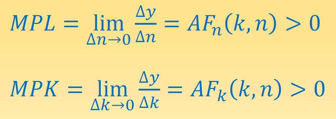
marginal productivity 遞減
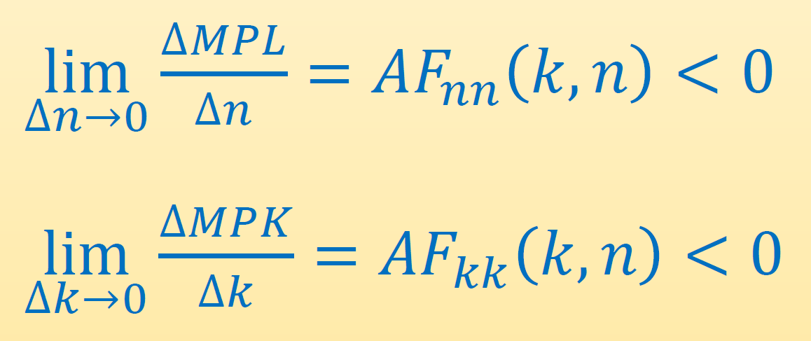
- 廠商規模未成熟時可能 MP 遞增,但這種情況不會持續存在
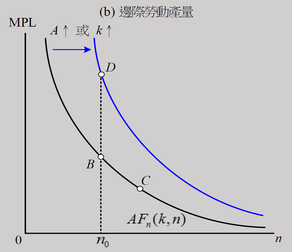
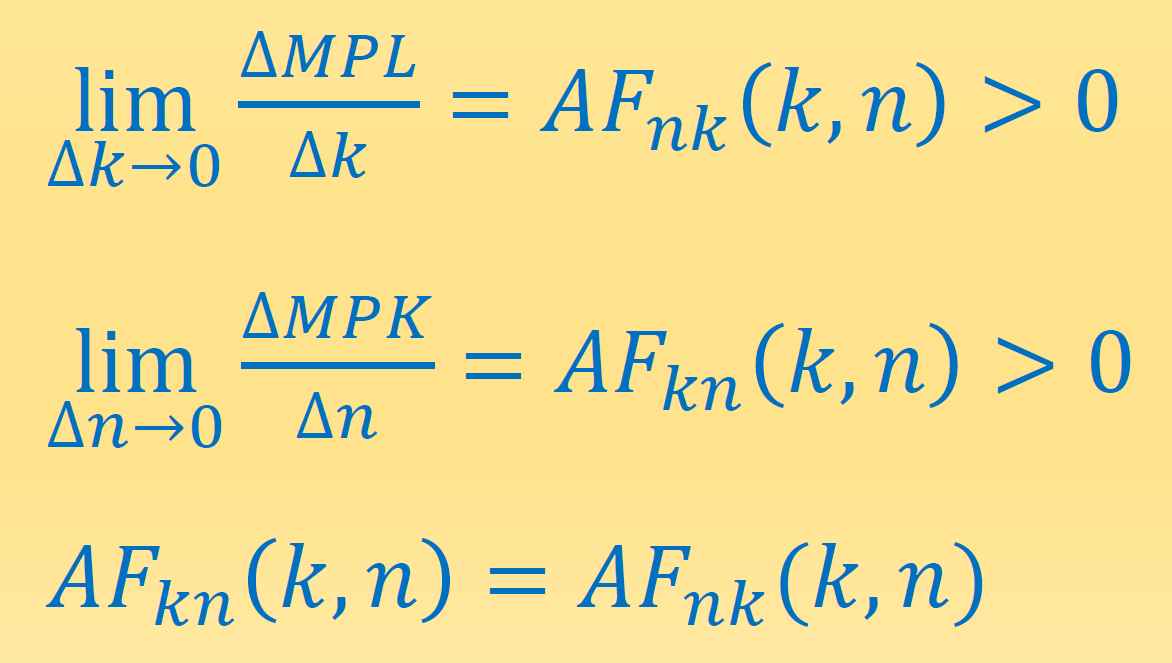
資本勞動互補
- capital 增加 → MPL 增加,反之亦然
Inada condition
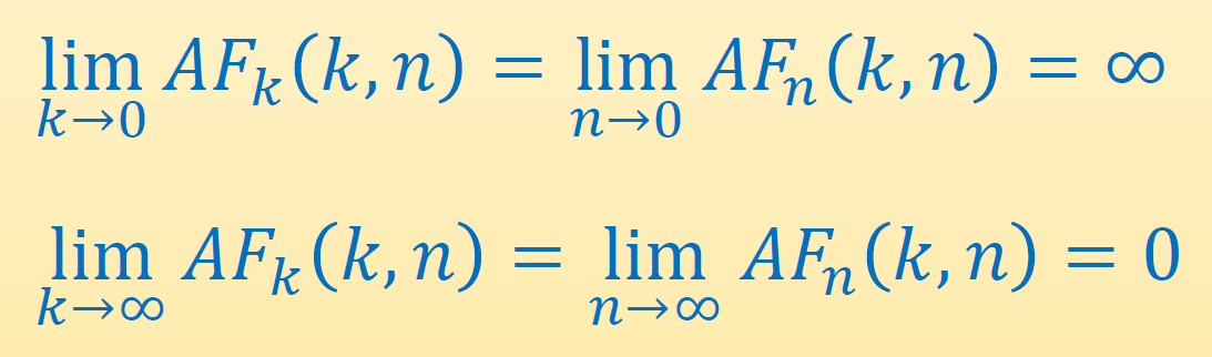
- 非必要條件
固定規模報酬 constant return to scale
- 生產效率 independent to 廠商規模
- 資本勞動皆 x2 → output x2
- 一階齊次函數
- 大公司切成 10 個小公司 → 生產效率不變
- 資本勞動皆 x2 → output x2
- \(AF(ak,an)>ay\) → 規模報酬遞增 increasing return to scale
- e.g. 台GG
- \(AF(ak,an)=ay\) → 規模報酬固定 constant return to scale
- \(AF(ak,an)<ay\) → 規模報酬遞減 decreasing return to scale
- e.g. 精緻餐廳、文創
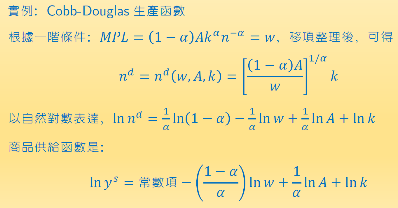
Cobb-Douglas 生產函數
- 要素產出彈性 output elasticity factor
- output 之於 factor 的彈性
- 資本產出彈性 = \(\dfrac{dy/y}{dk/k}\)
\(=\dfrac{d\ln y}{d\ln k}\)
\(=\dfrac{dy/dk\cdot k}{y}=\dfrac{MPK\cdot k}{y}=\dfrac{capital \space income}{output}\)
= 資本份額 capital share
- \(MPK=\dfrac{dy}{dk}=\alpha Ak^{\alpha-1}n^{1-\alpha}=\alpha \dfrac{y}{k}\)
- so \(\alpha\) = 資本產出彈性 = capital share = constant
- labor share = \(1-\alpha\) = constant
- 滿足 6 特性
Euler 性質
#固定規模報酬 constant return to scale
→ \(ay\equiv AF(ak,an)\)
→ \(\dfrac{d(ay)}{da}=y=AF_k(ak,an)\cdot k+AF_n(ak,an)\cdot n\)
\(=MPK\cdot k+MPL\cdot n\) for \(a=1\) (see #投入愈多,產出愈多)
= capital income + labor income
i.e. 廠商生產全部被資本&勞動報酬瓜分掉
Decision Problem
- 目標:max dividend
- dividend (profit) = revenue - cost
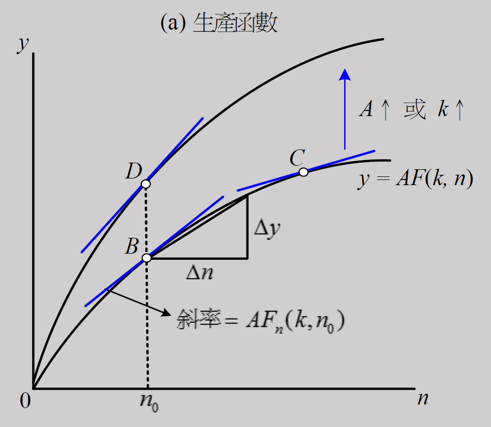
- \(d(n;A,k,w)=AF(k,n)-wn\)
- 一階必要條件
- \(AF_n(k,n^*)=w\) i.e. marginal profit = 0
- 二階充分條件
- \(AF_{nn}(k,n^*)<0\) i.e. MPL 遞減
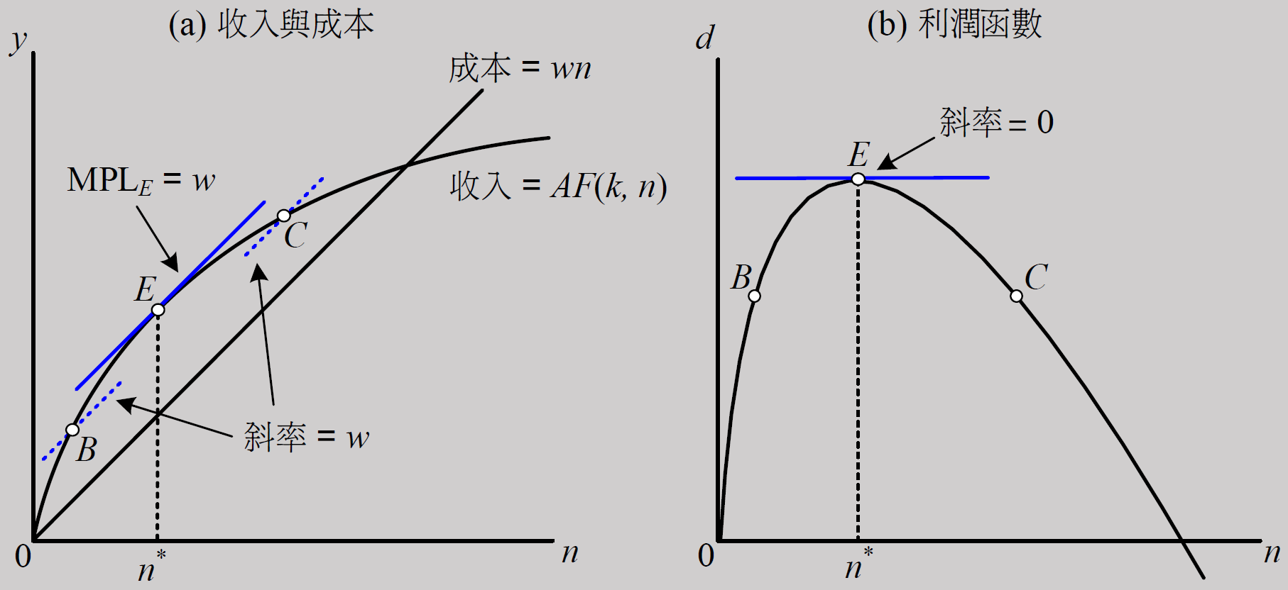
- \(MPL<w\) → d 遞增
- \(MPL>w\) → d 遞減
- \(MPL=w\) → d has max
labor & supply
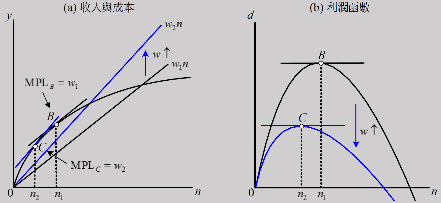
- wage
- w increase → n decrease
- A or k
- A or k increase → MPL increase → n increase
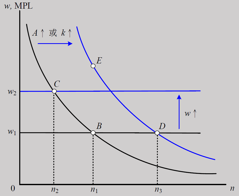
- B → wage increase → C
- B → A or k increase → D
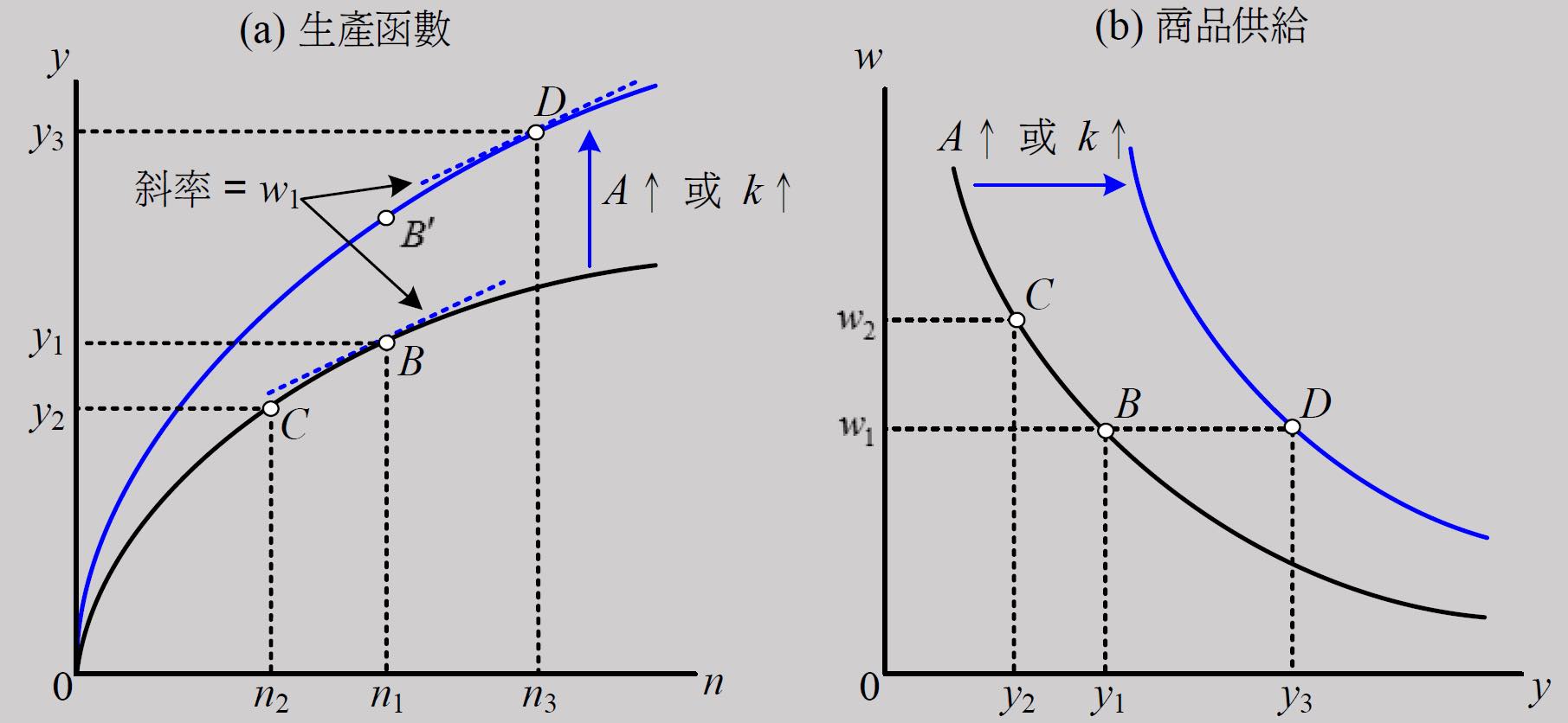
- B → wage increase → C
- B → A or k increase → D
- supply & demand
- labor demand \(n^d(w,A,k)\)
- w: negative
- A & k: positive
- product supply \(y^s(k,n^d(w,A,k))\)
- w: negative
- A & k: positive
- labor demand \(n^d(w,A,k)\)
能源危機
- 中間投入價格上升 → → MPL & MPK 下降
- \(y=F(k,n,x)\)
- x = 原油量
- q = 原油價格
- \(d(n,x)=F(k,n,x)-(wn+qx)\) 求 max
- 一階條件
- \(MPX=F_x(k,n,x)=q\)
- \(MPL=F_n(k,n,x)=w\)
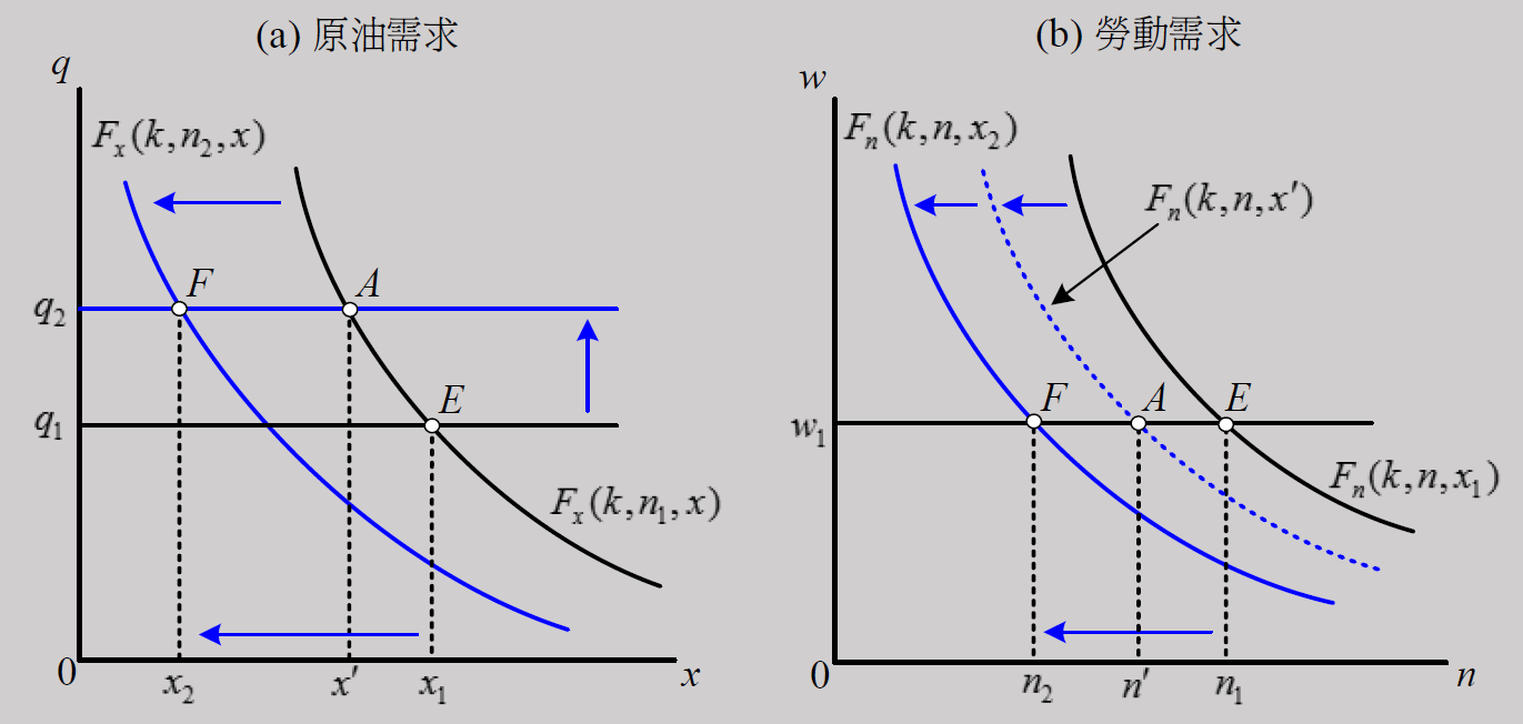
- 原油價格上升 → E to F,原油 & 勞動需求下降,商品供給下降, just like A 下降的結果
- q 上升 → x 下降 → MPL 下降 → labor demand 左移 → n 下降 → MPX 下降 → 原油 demand 左移 → x 下降
- 原油價格上升 → E to F,原油 & 勞動需求下降,商品供給下降, just like A 下降的結果
Cobb-Douglas 生產函數
- \(MPL=w=\beta\dfrac{y}{n}\)
- \(MPX=q=(1-\alpha-\beta)\dfrac{y}{x}\)
- 把 x 取代掉
- \(y=\left(\dfrac{1-\alpha-\beta}{q}\right)^{\frac{1-\alpha-\beta}{\alpha+\beta}}k^{\frac{\alpha}{\alpha_\beta}}n^{\frac{\beta}{\alpha_\beta}}=A_1k^{\phi}n^{1-\phi}\)
- q 上升 → \(A_1\) 下降 → MPL & MPK 下降
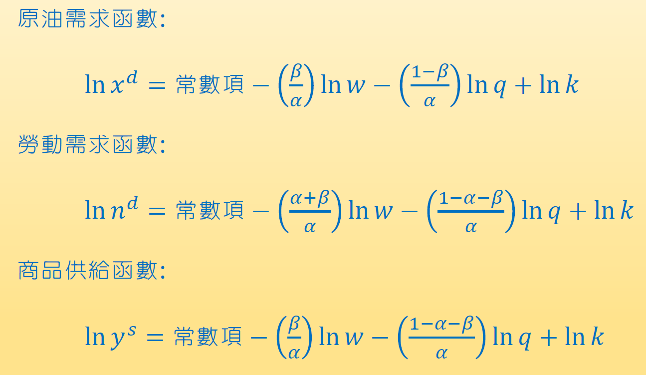
- q 上升 → \(x^d\) & \(n^d\) & \(y^s\) 下降
Ch5 消費者的靜態選擇
constraints
- time constraint
- l (leisure hours) + n (working hours) = 1
- income constraint
- c (商品消費) = a (非勞動所得) + wn (勞動所得)
- a (非勞動所得) = d (dividend) - T (定期稅淨額)
- c (商品消費) = a (非勞動所得) + wn (勞動所得)
- budget constraint
- x = c + wl = a + w = full income
- wl 相當於花費於 leisure 的錢
- w = wage = 每時間單位的 leisure 的 opportunity cost
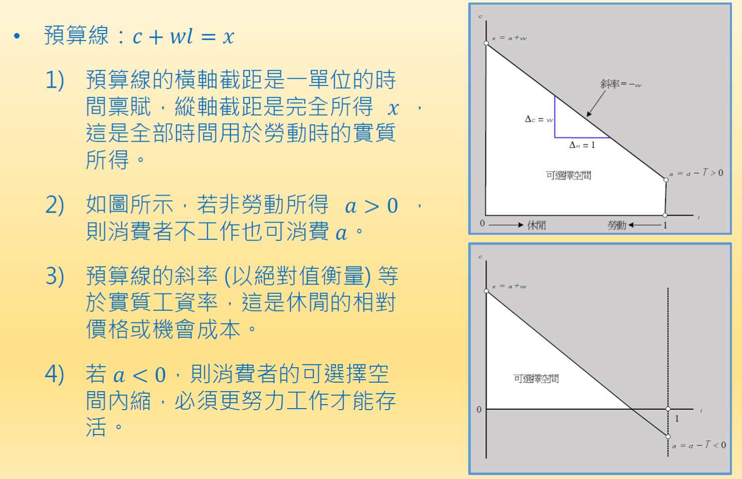
- a 增加 → 向上平移
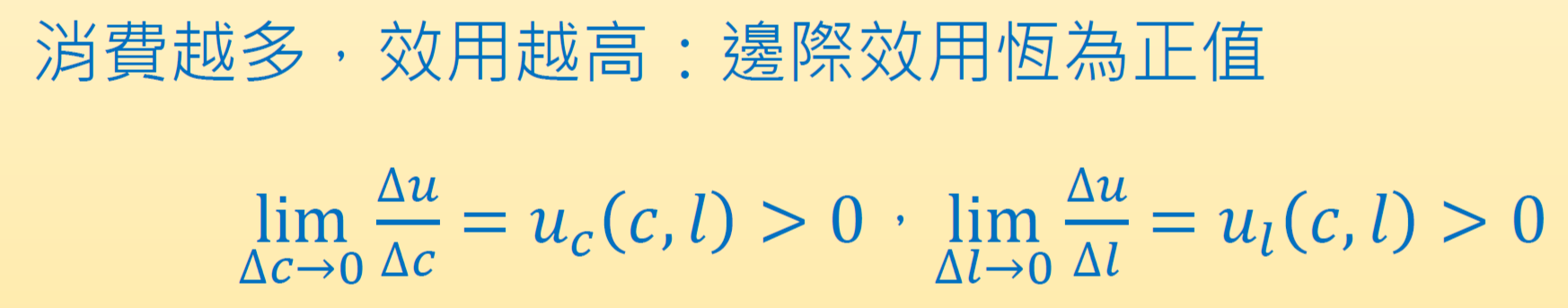
utility function
- assumptions
- marginal utility > 0
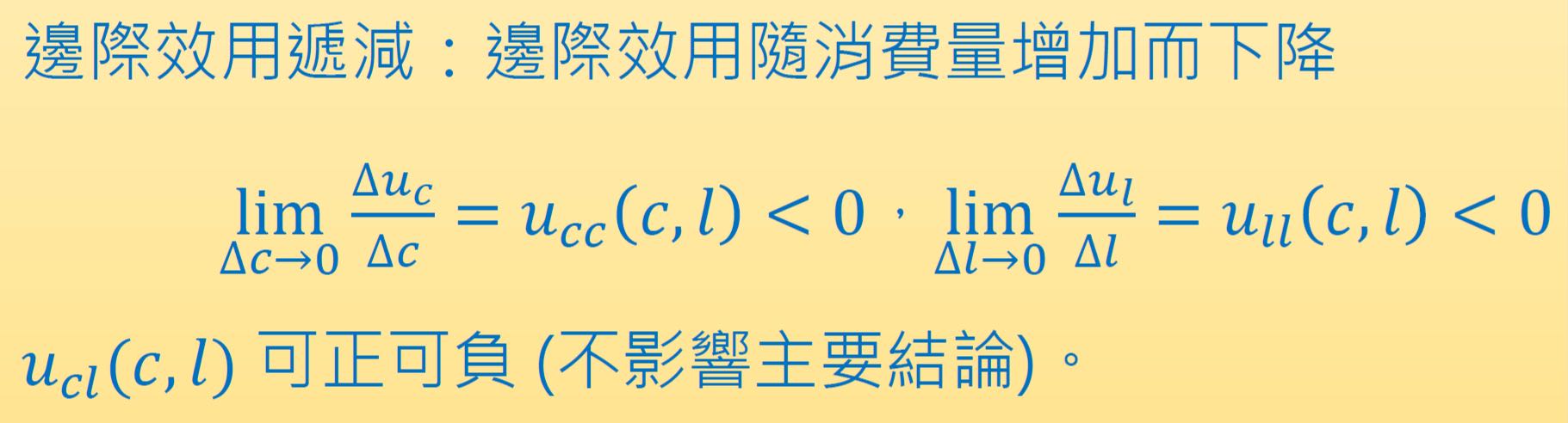
- marginal utility 遞減
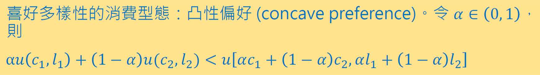
- concave preference
- 凹函數
- c & l \(\in\) normal goods
- 消費 & leisure 都是 normal goods
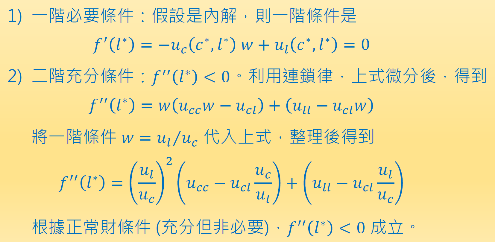
- sufficient conditions
- \(u_{cc}-u_{cl}\dfrac{u_c}{u_l}<0\)
- \(\dfrac{u_{cc}}{u_{cl}}<\dfrac{u_c}{u_l}\)
- \(u_{ll}-u_{cl}\dfrac{u_l}{u_c}<0\)
- \(u_{cc}-u_{cl}\dfrac{u_c}{u_l}<0\)
- marginal utility > 0
- indifference curve
- \(MRS_{l,c} = \dfrac{u_l}{u_c}=w\)
- homothetic preference 同位偏好
- \(u(ax,ay) = au(x,y)\)
- x y 比值相同 → MRS 相同
- solution
- budget constraint \(c=a+wn=a+w(1-l)\) → \(c+wl=a+w\)
- \(u_c(c^*,l^*)w=u_l(c^*,l^*)\)
\(w=\dfrac{u_l(c^*,l^*)}{u_c(c^*,l^*)}\)- 休閒取代消費的邊際效益 (MR) = wage (MC)
- work 1 time unit more → lose \(u_l\) more utility but get w more money → consume w more money → get \(wu_c\) more utility
- w 上升 → leisure 變貴 → budget line 變陡
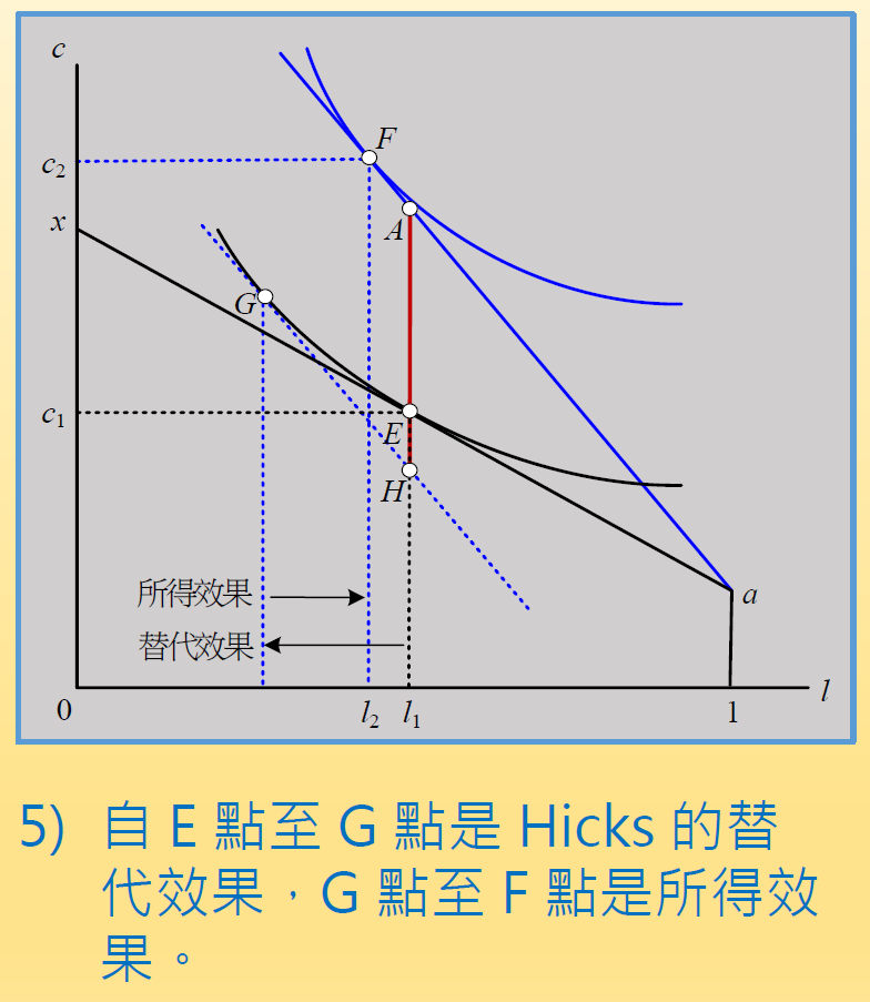
- Hicks

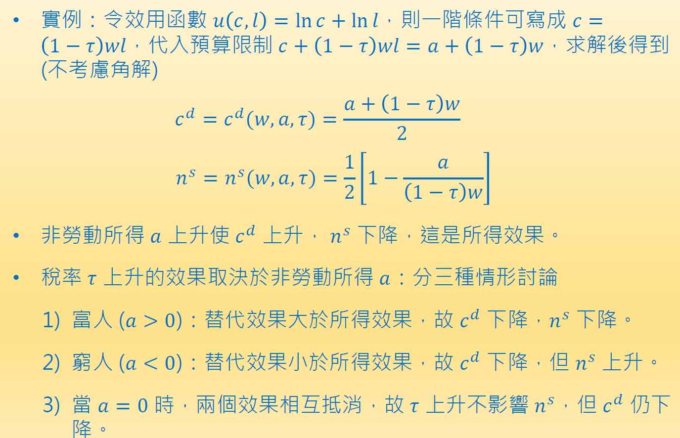
勞動所得稅
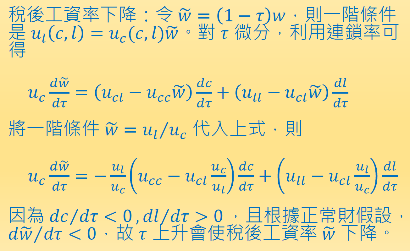
- 勞動所得稅率 \(\tau\)
- real wage w → \((1-\tau)w\)
- leisure 變便宜 → 消費 demand 降低 (substitution effect)
- 非勞動所得 > 0 (rich) → substitution effect 較大 → 減少工時 (\(n^s\))
- 非勞動所得 < 0 (poor) → income effect 較大 → 增加工時
消費券 consumption voucher
- 為 transfer payment
- 既是消費也是支出(一定需要花掉) → 左右相消,不影響 budget constraint
- 會使 \(MRS_{l,c}\) 上升,leisure 意願上升,消費&勞動意願下降

- \(u_{cc}-u_{cl}\dfrac{u_c}{u_l}<0\) 是 normal good 的必要條件

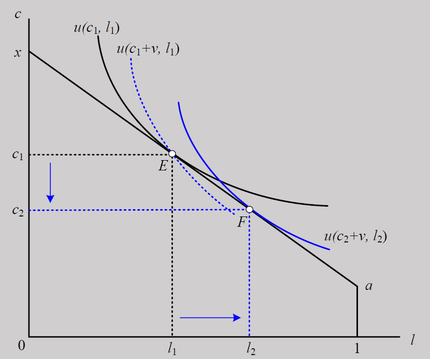
- endowment = E
- got voucher \(v\) → MRC i.e. slope of indifference curve increase, budget line stays the same → new equilibrium F
- \(c_2<c_1\) but \(c_2+v>c_1\)
- 所謂 budget line 不變是在 c 已經減掉了 \(v\) 的情況下,不然其實是 budget line 上移,indifference curve 穿過 \(c_1+v\),於是移到新均衡 where indifference curve 切 new budget line
Ch6 靜態模型的全面均衡
Walras Law of Markets

- 商品市場超額需求 + 勞動市場超額需求 = 0
- 薪資水準低 → 消費需求低,勞動供給高 (?)
競爭均衡三面向
第一面向-連立方程解
第二面向-市場供需模型
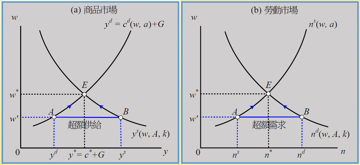
- w' < w* → 勞動超額需求 → w 上升 直到 E 點
第三面向-通吃型圖形
- 全面均衡
- 生產可能線 PPF
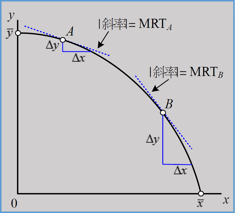
- x y 兩產品
- 可生產 x or y
- 邊際生產力遞減 → y 很多,x 很少時,消耗一些 y 的生產力,減少一點 y,能夠多生產很多 x → 凸
- MRT = \(\dfrac{\Delta y}{\Delta x}\)
- MRT 隨 x 遞增
- 價格調整
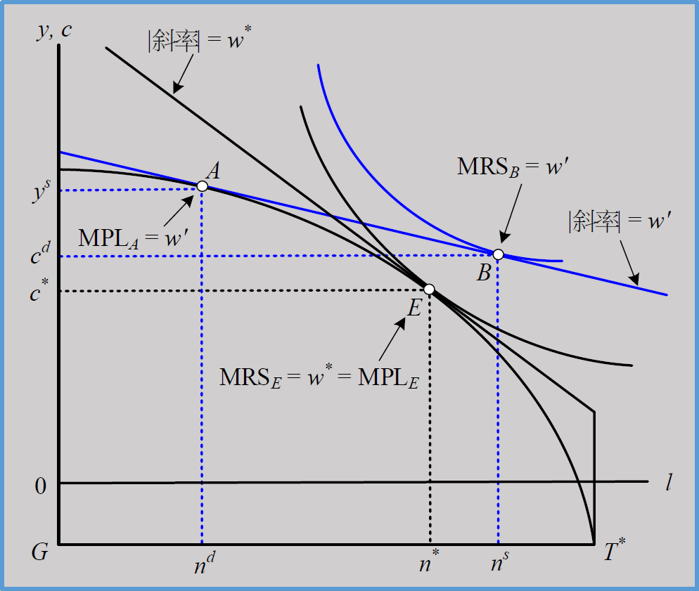
- w' → 超額勞動需求,超額商品供給 → w 上升 to w → 廠商 & 消費者 converge to E 點,MPS = MPS = w
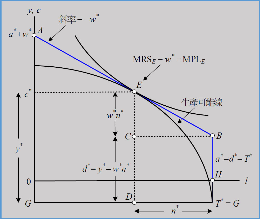
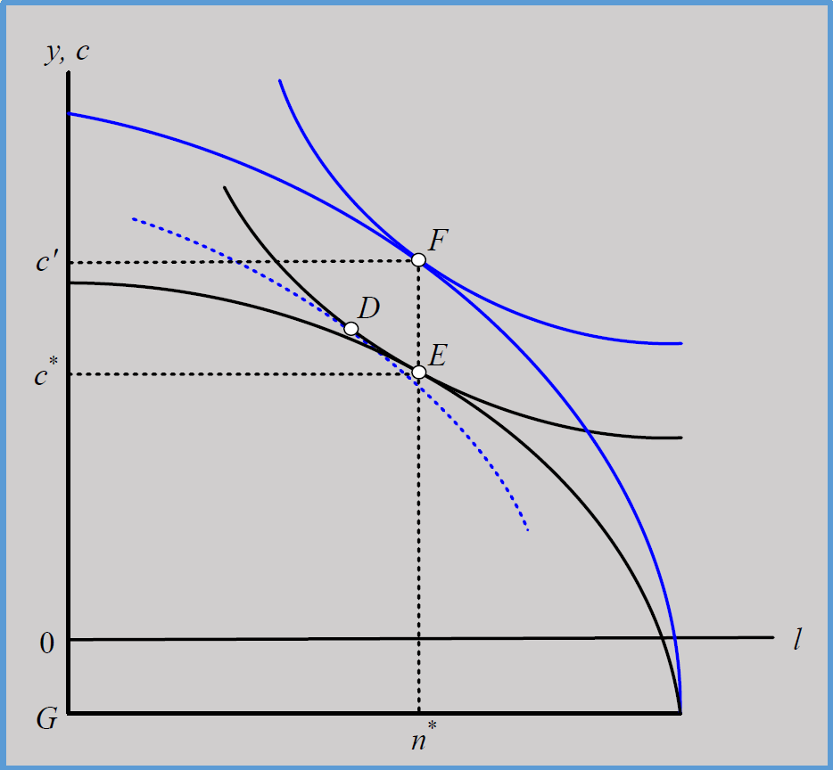
Crusoe 荒島經濟
- Crusoe 同時為消費者 & 生產者
- 生產&消費椰果 all by himself

- G 是 loss of 椰果 for whatever reason
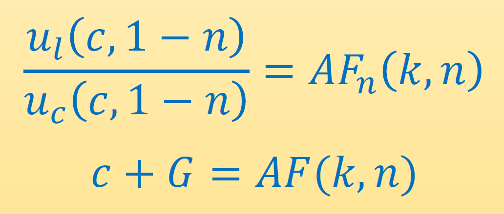
- \(u_l(c^*,l^*)=u_c(c^*,l^*)AF_n\)
\(MRS_{l,c}=\dfrac{u_l}{u_c}=AF_n=MPL\)- MPL = \(AF_n\) = 設算價格 imputed price / 影子價格 shadow price,即市場的 real wage
- work 1 time unit more → lose \(u_l\) more utility but get MPL more coconuts → consume w more coconuts → get \(MPL\times u_c\) more utility
- 與市場經濟的不同
- 消費者生產量會決定 leisure 的 cost
- 這裡的 pareto optimum 是效益最大化那個唯一解,因為只有一個人要考慮
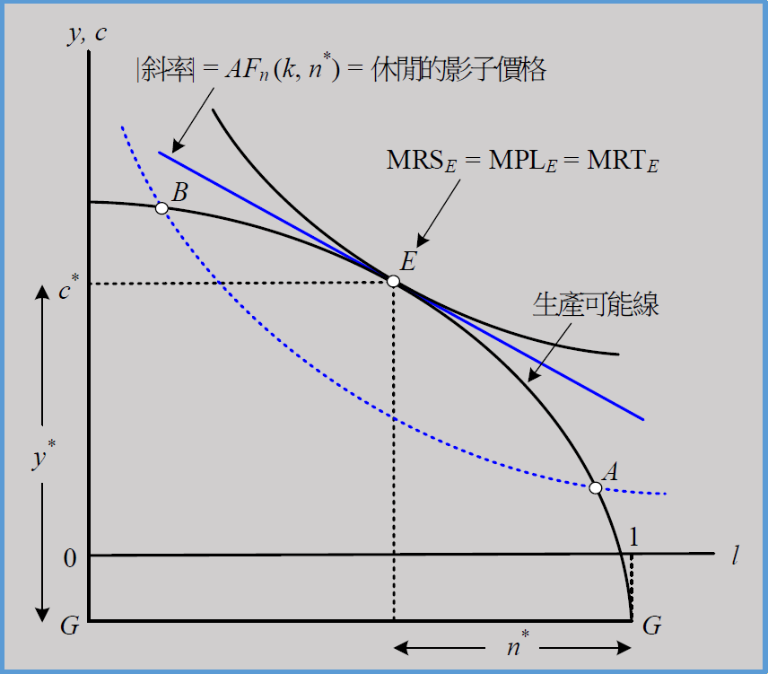
- A: MPL > MRS
- B: MPL < MRS
- E: MRS = MPL
- slope = leisure's 影子價格
- competitive equilibrium 即為 pareto optimum
福利定理
- first welfare theorem
- in perfect competition, equilibrium will be Pareto optimal
- second welfare theorem
- any Pereto optimum can be achieved as the competitive equilibrium for some endowment distribution
- pf with Edgeworth box
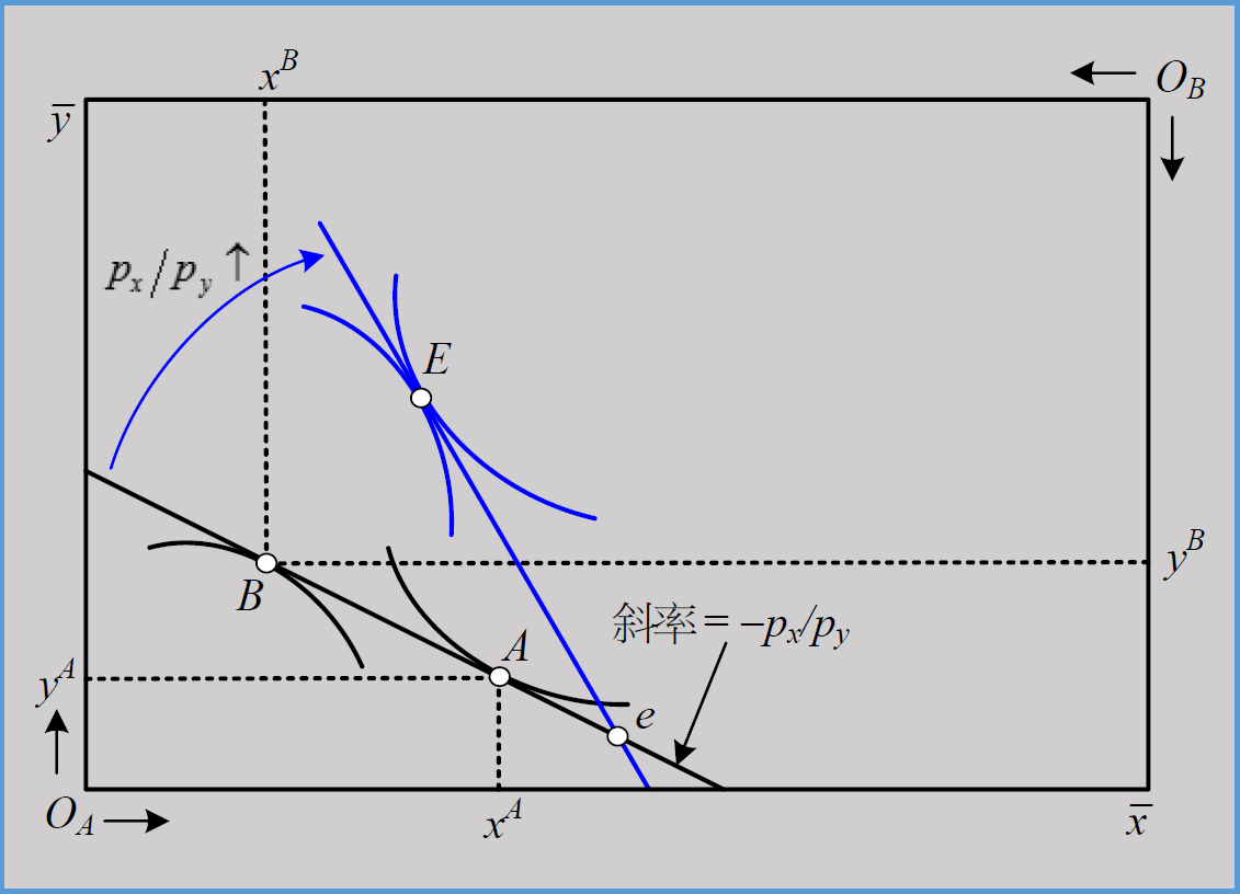
- at the optimal solutions of the budget line on endowment point e
- \(x^A+x^B>\bar{x}\) → demand > supply
- \(y^A+y^B<\bar{y}\) → demand < supply
- so \(p_x\) increase, \(p_y\) decrease, \(\dfrac{p_x}{p_y}\) increase,until x&y's solutions meet
- at the optimal solutions of the budget line on endowment point e
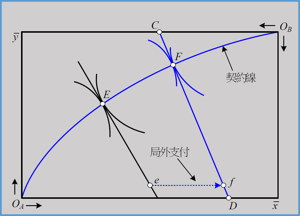
- 在 contract curve 以外的點都存在 mutually advantage area → converge 到 contract curve while maintaining Pareto → first welfare theorem
- to achieve a certain point in the contract curve i.e. a certain Pareto optimal solution, just redistribute the endowment points, e.g. all endowment points on line CD will converge to point F → second welfare theorem
市場均衡的不效率性
- irl 使 equilibrium 非 pareto optimal 的因素
- 存在外部性 → 存在改善空間
- marginal private cost < marginal social cost
- e.g. 汙染
- marginal private gain < marginal social gain
- e.g. 不同工同酬
- marginal private cost < marginal social cost
- information incomplete/asymmetric
- extra cost for information → deadweight loss
- agency problem
- 扭曲性租稅 distorting taxes
- model 用定額稅 i.e. 人頭稅,not a function of labor time → won't affect wage → won't affect choice between consumption & leisure
- irl 不會用人頭稅,是會影響生產者 or 消費者選擇的 distorting taxes
- monopoly power of firms
Ch7 靜態模型的均衡分析
政府消費支出增加
- for Crusoe
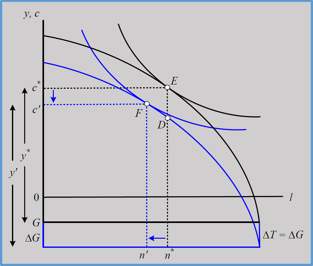
- 政府消費增加 → 政府定額稅增加 → 等效於 G 增加
- 不影響 MPL → slope unchanged for any n
- E to F
- leisure 下降,coconuts i.e. 商品供給上升
- consumption i.e. 商品需求下降 (income effect)
- MPL i.e. real wage 下降
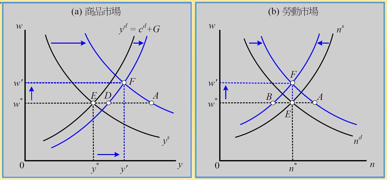
- for market
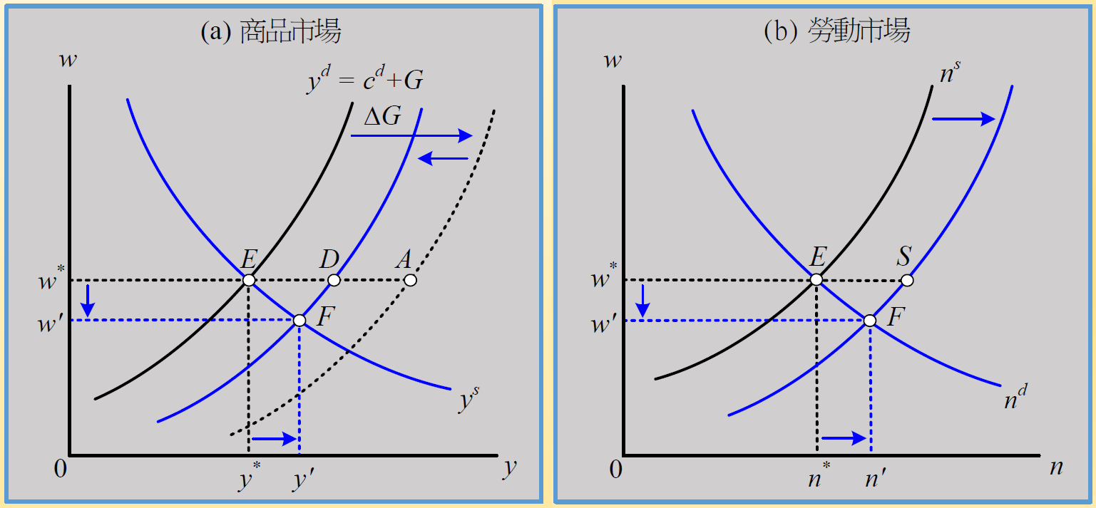
- 直接效果
- G 上升 → \(y^d\) shift right (E to A)
- income effect
- 定額稅上升 → 非勞動所得下降 → leisure & consumption demand 下降,labor supply 上升 → \(y^d\) shift left (A to D), \(n^s\) shift right (E to S)
- income effect 的 y shift left 幅度 < 直接效果的 y shift right 幅度 → end in EA 之間
- c+wl = w+(d-T) → \(\Delta c+w\Delta l=\Delta T\) for w & d unchanged → \(\Delta c<\Delta T\)
- 如果 y shift left 幅度較大,end with w'>w* in 商品市場,則商品&勞動市場皆存在超額供給 → 違反 #Walras Law of Markets
- 工資效果
- at w*,商品市場出現超額需求 (ED),勞動市場出現超額供給 (ES) → w 下降
- → 商品供給上升 & 勞動需求上升 (E to F)
- → leisure 變便宜 (substitution effect) → 商品需求下降 (D to F) & 勞動供給下降 (S to F)
- at w*,商品市場出現超額需求 (ED),勞動市場出現超額供給 (ES) → w 下降
- income effect & substitution effect 均使 consumption demand 下降
- income effect 使 labor supply 上升幅度 > substitution effect 使 labor supply 下降幅度,最終 E to F,勞動量 & 生產量上升
- 因為 wage 降低,廠商 hire more
- 與 Crusoe model 一致
- 結論
- 排擠效果
- 政府支出使消費者均衡消費量下降 i.e. 政府消費排擠民間消費
- y = c + G → \(\Delta y=\Delta c+\Delta G\),又 G 上升會使 c 減少 → \(\Delta y<\Delta G\)
- 政府消費性支出使消費者 utility 下降
- 勞動增加、消費減少、工資減少
- 政府支出會使產出&就業增加,但會使消費&實質工資下降,so 政府支出不是造成景氣波動的主因
- 模型的缺陷
- 有些政府支出能替代民間消費 → 提升消費者 utility
- e.g. 營養午餐、治安
- 公共工程會刺激民間生產 (?)
- 有些政府支出能替代民間消費 → 提升消費者 utility
- 排擠效果
供給面衝擊
- A (TFP) 上升
- for Crusoe
- MPL increase → leisure more expensive → E to D (substitution effect)
- more coconuts → D to F (income effect)
- 消費量&生產量上升
- labor amount 方向不一定
- for market
- 直接效果
- A increase → MPL increase → labor demand (\(n^d\)) & goods supply (\(y^s\)) increase
- \(\Delta d=F\Delta A\) i.e. dividend increase = A 上升的直接效果
- \(\Delta y^s=F\Delta A+MPL n^d\)
- \(\Delta d=\Delta y^s-w\Delta n^d\)
- \(\Delta d=F\Delta A+(MPL-w)\Delta n^d\)
- \(MPL = w\)
- income effect
- A increase → consumer dividend increase → consumption demand (\(y^d\)) increase & leisure demand increase i.e. labor supply (\(n^s\)) decrease
- income effect 的 \(y^d\) shift right 幅度 < 直接效果的 \(y^s\) shift right 幅度 (ED<EA)
- c+wl = w+(d-T) → \(\Delta c+w\Delta l=\Delta d\) for w & T unchanged → \(\Delta c<\Delta d\)
- 工資效果
- 在 w*,goods market 超額供給,labor market 超額需求
- wage increase
- → consumption demand (\(y^d\)) increase (D to F) & labor supply (\(n^s\)) increase (B to F)
- → goods supply (\(y^s\)) decrease (A to F) & labor demand (\(n^d\)) decrease (A to F)
- 結論
- A 上升 → production & consumption & wage 上升,labor 不一定
計算實例
- 給定
- \(u=\ln c+\ln l\)
- \(y=An^{\alpha}, \alpha\in(0,1)\)
- \(G=gy=T\)
- \(g\) = 政策變數,表政府支出佔總產出的比例
- \(c=y-G=y-gy=y(1-g)\)
- 均衡條件
- \(MRS=\frac{u_l}{u_c}=\frac{c}{l}=\frac{(1-g)y}{1-n}=MPL=y_n=\frac{\alpha y}{n}\)
- 解得
- \(n=\frac{\alpha}{1+\alpha-g}\)
- \(y=An^{\alpha}=A(\frac{\alpha}{1+\alpha-g})^{\alpha}\)
- \(c=(1-g)y=(1-g)A(\frac{\alpha}{1+\alpha-g})^{\alpha}\)
- \(w=MPL=\frac{\alpha y}{n}=\alpha A(\frac{1+\alpha-g}{\alpha})^{1-\alpha}\)
- A 不影響 n
- u & y 使 A 變動產生的 income effect & substitution effect 剛好抵銷
- y, c, w 接隨 A 上升
- n 隨 g 上升
- \(\frac{d\ln c}{dg}=\frac{-1}{1-g}+\frac{\alpha}{1+\alpha-g}=\frac{(1-\alpha)g-1}{(1-g)(1+\alpha-g)}<0\)
- g 上升會使 c 下降
勞動所得稅
- \(\tau\) = 所得稅率
- \(G=T+\tau wn\) = 定額稅+所得稅
- \(c=(d-T)+(1-\tau)wn\) = 非勞動所得+勞動所得
- \(MRS=\frac{u_l}{u_c}=(1-\tau w)\)
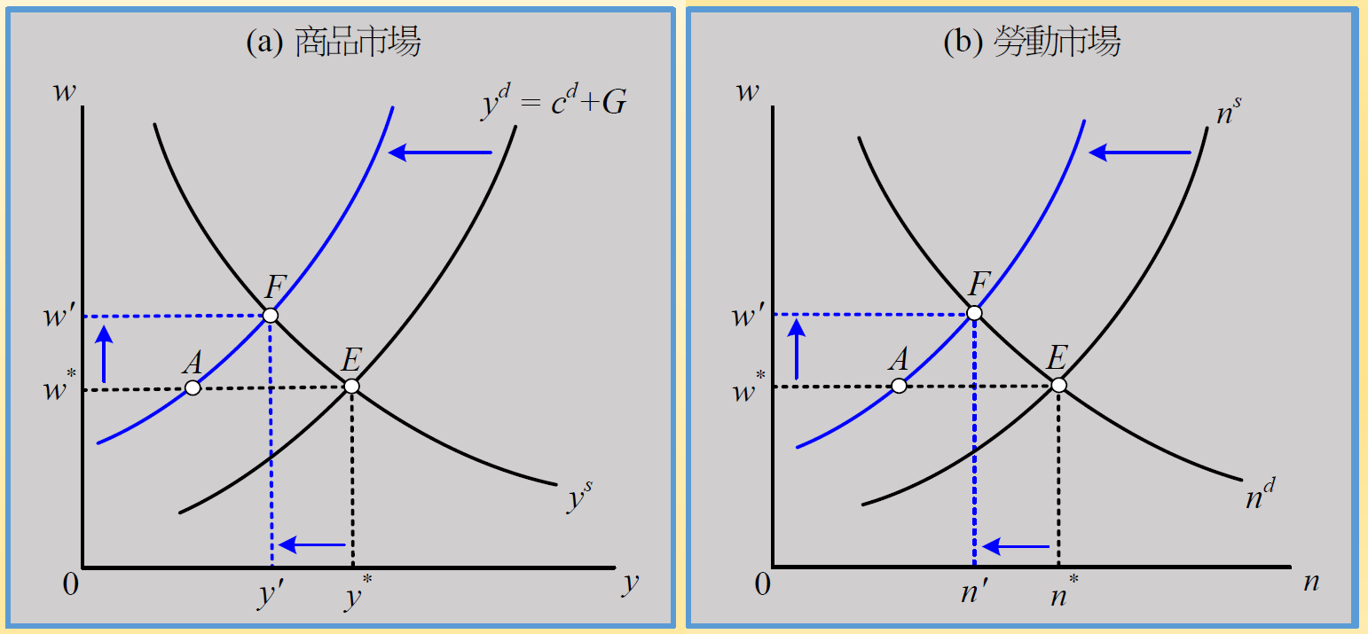
- 稅率 \(\tau\) 上升
- substitution effect → consumption demand (\(c^d\)) & labor supply (\(n^s\)) 下降 bc
- 廠商最適選擇不變 → \(n^d\) & \(y^s\) 不動
- → 在原 wage,商品市場超額供給,勞動市場超額需求 → 移動到新均衡 F,(稅前) wage 上升
- 稅前工資率上升,but 稅後工資率是下降
- 稅前工資率上升,but 稅後工資率是下降
- 市場結清條件
- \(c^d+G=y\)
- \(n^d=n^s\)
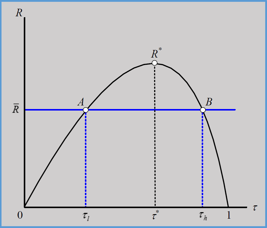
- Laffer curve
- 背景 (1980s)
- 經濟不景氣
- 雙赤字問題 twin deficits
- 貿易逆差
- 預算赤字
- 供給面經濟學 / 雷根經濟學
- 降低稅率 → 刺激景氣&增加總稅收
- \(R=\tau wn\)
- overall tax revenue
- \(\tau\) 上升 → (稅前) w 上升,n 下降
- \(\ln R=\ln \tau+\ln w+\ln n\)
- if w 不變,\(\frac{d\ln R}{d\ln \tau}=1+\frac{d\ln n}{d\ln \tau}=1-\eta_{\tau}\)
- \(\eta_{\tau}\) = 勞動供給的稅率彈性
- \(\eta_{\tau}<1\) → R 隨 \(\tau\) 上升
- \(\eta_{\tau}>1\) → \(\tau\) 上升使 R 下降
- \(\tau\) 上升,稅後 w 下降幅度變大
- 總稅收 R vs. 稅率 \(\tau\) (if w 不變)
- 背景 (1980s)
- 全面均衡 (考慮 w)
- 令 \(u=\ln l+\ln c\) && \(y=n^\alpha\)
- \(MRS=\dfrac{c}{1-n}=(1-\tau)w=(1-\tau)MPL=(1-\tau)\dfrac{\alpha y}{n}\)
- \(w=MPL=\dfrac{\alpha y}{n}\)
- \(n=\dfrac{\alpha (1-\tau)}{1+\alpha(1-\tau)}\in(0,1)\)
- \(R=\tau wn=\tau\alpha y=\tau\alpha {\left[\dfrac{\alpha (1-\tau)}{1+\alpha(1-\tau)}\right]}^\alpha\)
消費券均衡效果
- 消費券會替代部分私人消費 & 使勞動供給下降,but 總消費量仍增加
- 均衡條件
- \(MPL = f'(n) = w\)
- 廠商利潤極大
- 不受 voucher 影響
- \(MRS=\frac{u_l}{u_c}=(1-\tau)w\)
- 消費者效用極大
- \(c+v=\tilde{c}=y=f(n)\)
- 市場結清條件
- \(v=T+\tau wn\)
- 政府預算均衡
- \(MPL = f'(n) = w\)
- 消費券有中立性質
- 前三項均衡解與 \(v\) 無關
- \(v\) 不影響產出、勞動、市場工資率 → 私人消費完全被排擠
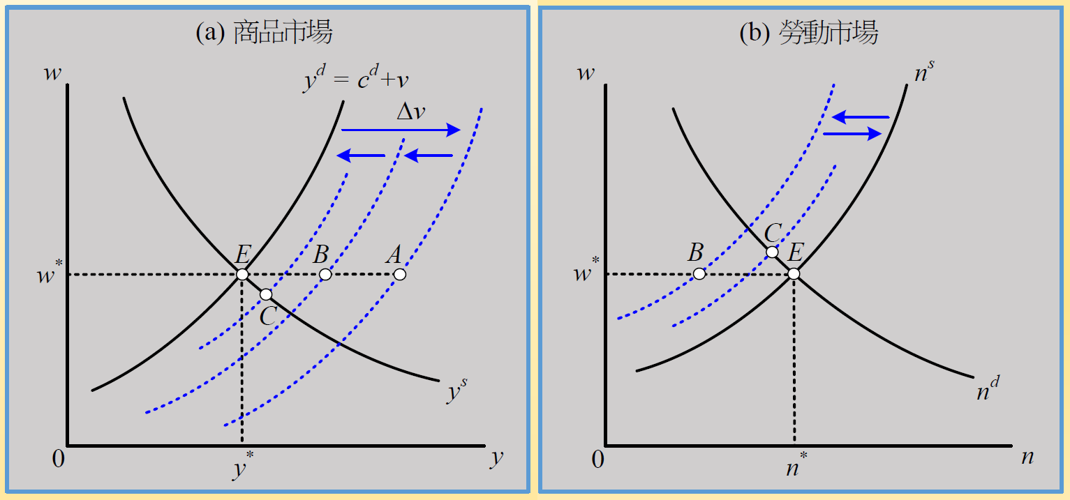
- 直接效果
- 商品需求 \(y^d\) 右移 E to A
- substitution effect
- 消費券替代部分私人消費
- 商品需求 \(y^d\) 左移 A to B
- labor supply \(n^s\) 左移 E to B
- income effect
- 定額稅增加 EA → 商品需求 \(y^d\) 左移
- labor supply \(n^s\) 右移
- income effect 幅度不可能同時大於 or 小於 substitution effect,否則會陷入不均衡狀態 → 必回到原均衡點 E
- e.g. C 點與原點 E 比, labor supply 下降,comsumption demand 卻上升
- so 定額稅融通消費券具中立性質,對整體經濟毫無影響
工時的長期趨勢
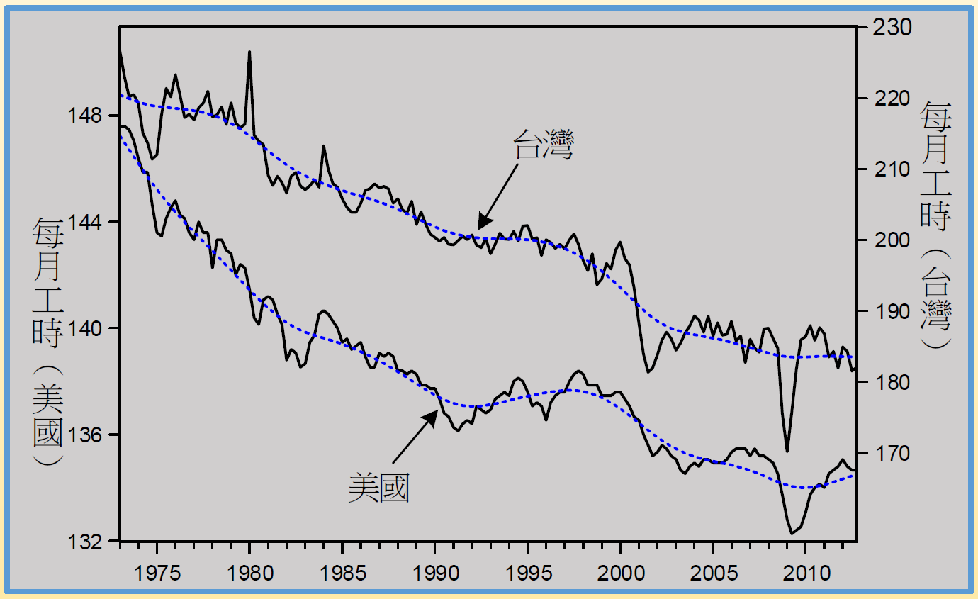
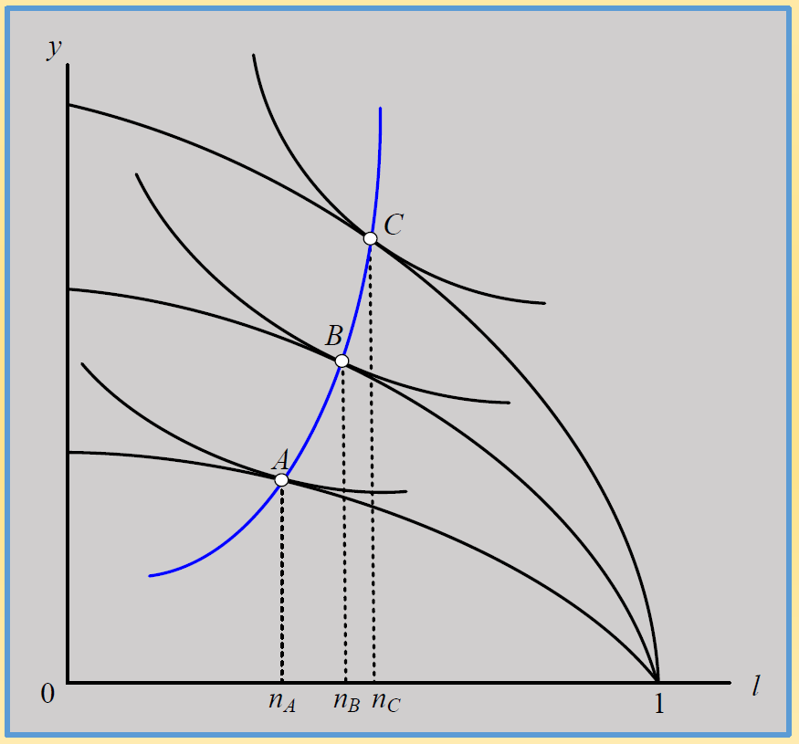
- 早期 PPF 較低,indifference curve 較平緩
- PPF 上升 → income effect & substitution effect
- income effect 使 labor 下降
- substitution effect 使 labor 上升
- for 窮人 (A → B),income effect 很強 → labor 下降 i.e. leisure 上升明顯
- for 較有錢的人 (B → C),substitution effect 抵銷 income effect → labor 下降 i.e. leisure 上升趨勢減緩
Ch8 消費與儲蓄
Notation
- \(a_t\) = t 期 endowment
- \(b_t\) = t 期 期初擁有 bonds
- \(c_t\) = t 期 consumption
- \(r_t\) = t 期 利率
- \(s_t\) = t 期 saving
- \(\beta\) = 1 期後的 1 單位的 utility 在今天的價值
- see #費雪兩期模型#utlity
費雪兩期模型
budget constraint
- Fisher Two-Period Model
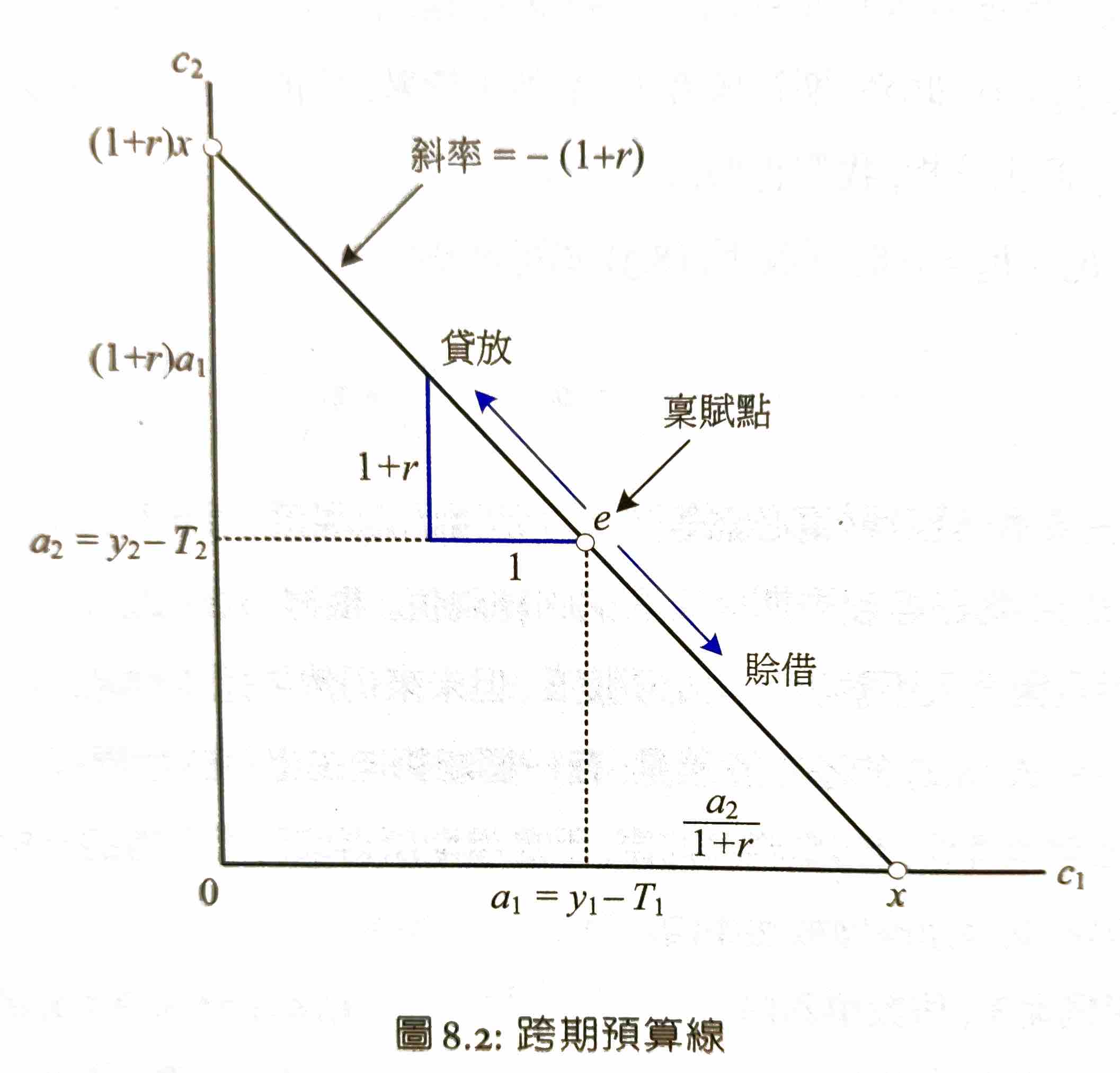
- \(a_1=y_1-T_1\) = 1st 期稅後 endowment
- \(a_2=y_2-T_2\) = 2nd 期稅後 endowment
- \(c_1+b_1=a_1+(1+r)b_0\)
- \(b_0\) = 1st 期期初擁有之債券,可為負數
- \(b_1\) = 1st 期期末債券餘額
- \(c_1\) = 1st 期可花的錢
- \(s_1=(a_1+rb_0)-c_1=b_1-b_0\)
- \(s_1\) = 1st 期 saving = 可支配所得 - 消費
- 債券本金 \(b_0\) 不是所得,而是原本就存著的
- \(c_2+b_2=a_2+(1+r)b_1\)
- \(b_1 = \dfrac{c_2+b_2-a_2}{1+r}\)
- lifetime wealth
- \(\left( c_1+\dfrac{c_2}{1+r}\right)+\dfrac{b_2}{1+r}=\left(a_1+ \dfrac{a_2}{1+r}\right)+(1+r)b_0\)
- 右邊 = lifetime wealth = 稅後 endowment 現值 + 期初債券本利和
- 左邊 = 兩期消費&期末債券餘額現值
- 消費者會追求 \(b_2=-\infty\) → 限制 \(b_2\geq 0\) → \(b_2=0\)
- 否則債券市場會直接關門
- \(b_0=b_2=0\) → \(c_1+\dfrac{c_2}{1+r}=a_1+\dfrac{a_2}{1+r}\equiv x\) = lifetime wealth
- lifetime wealth 決定消費者各期消費能力
- \(\left( c_1+\dfrac{c_2}{1+r}\right)+\dfrac{b_2}{1+r}=\left(a_1+ \dfrac{a_2}{1+r}\right)+(1+r)b_0\)
utlity
- 兩期消費 marginal utility > 0 且遞減
- MRS 遞減
- \(MRS_{12}=-\dfrac{d_{c_2}}{d_{c_1}}=\dfrac{U_1(c_1,c_2)}{U_2(c_1,c_2)}\)
- 兩期消費為正常財
- \(U_{11}-U_{12}\dfrac{U_1}{U_2}<0\)
- \(U_{22}-U_{12}\dfrac{U_2}{U_1}<0\)
- \(U(c_1,c_2)=u(c_1)+\beta u(c_2)\)
- 時間可分割性 & 時間可加性
- \(U_{12}=0\)
- 各期 utility independent to 他期消費水準
- time preference
- \(\beta\in(0,1)\) = 時間偏好因子
- \(\beta = \dfrac{1}{1+\rho}\), \(\rho>0\)
- \(\rho\) = 主觀利率 subjective interest rate
- utility 折現率
- 未來比今天爛,爛多少
- when \(c_1=c_2=c\),\(MRS_E=\dfrac{U_1(c,c)}{U_2(c,c)}=\dfrac{u'(c)}{\beta u'(c)}=\dfrac{1}{\beta}=1+\rho\)
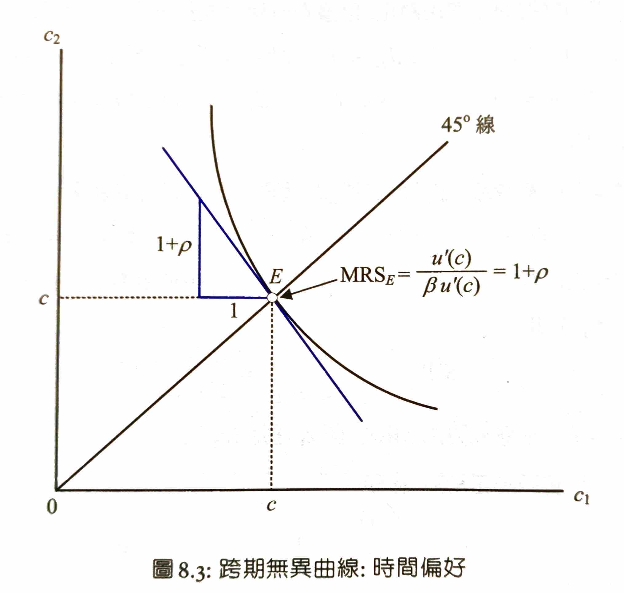
- 45 度線 indifference curve 切線斜率
choice
- budget constraint: \(c_1+\dfrac{c_2}{1+r}=a_1+\dfrac{a_2}{1+r}=x\)
- utility function: \(U(c_1,c_2)=u(c_1)+\beta u(c_2)\)
- 使 saving 的 marginal profit = 0
- \(u'(c_1)=\beta u'(c_2)(1+r)\)
- \(MRS_{12}=\dfrac{u'(c_1)}{\beta u'(c_2)}=1+r\)
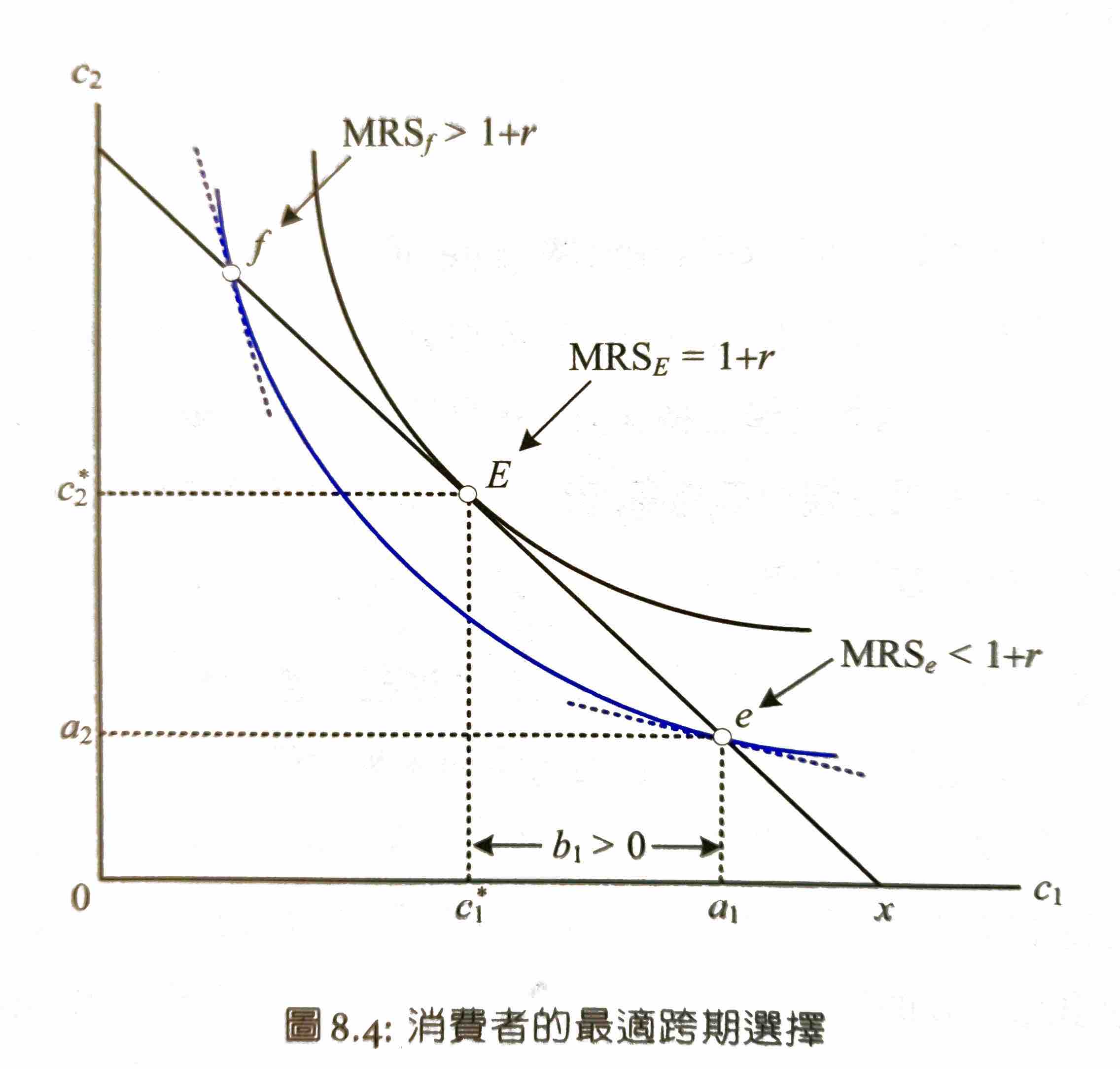
- MRS < 1+r → 儲蓄比消費爽 → 增加儲蓄
- MRS > 1+r → 消費比儲蓄爽 → 增加消費
- MRS = 1+r → 消費跟儲蓄一樣爽 → 均衡
所得變動 & 消費平滑
- 當期可支配所得增加
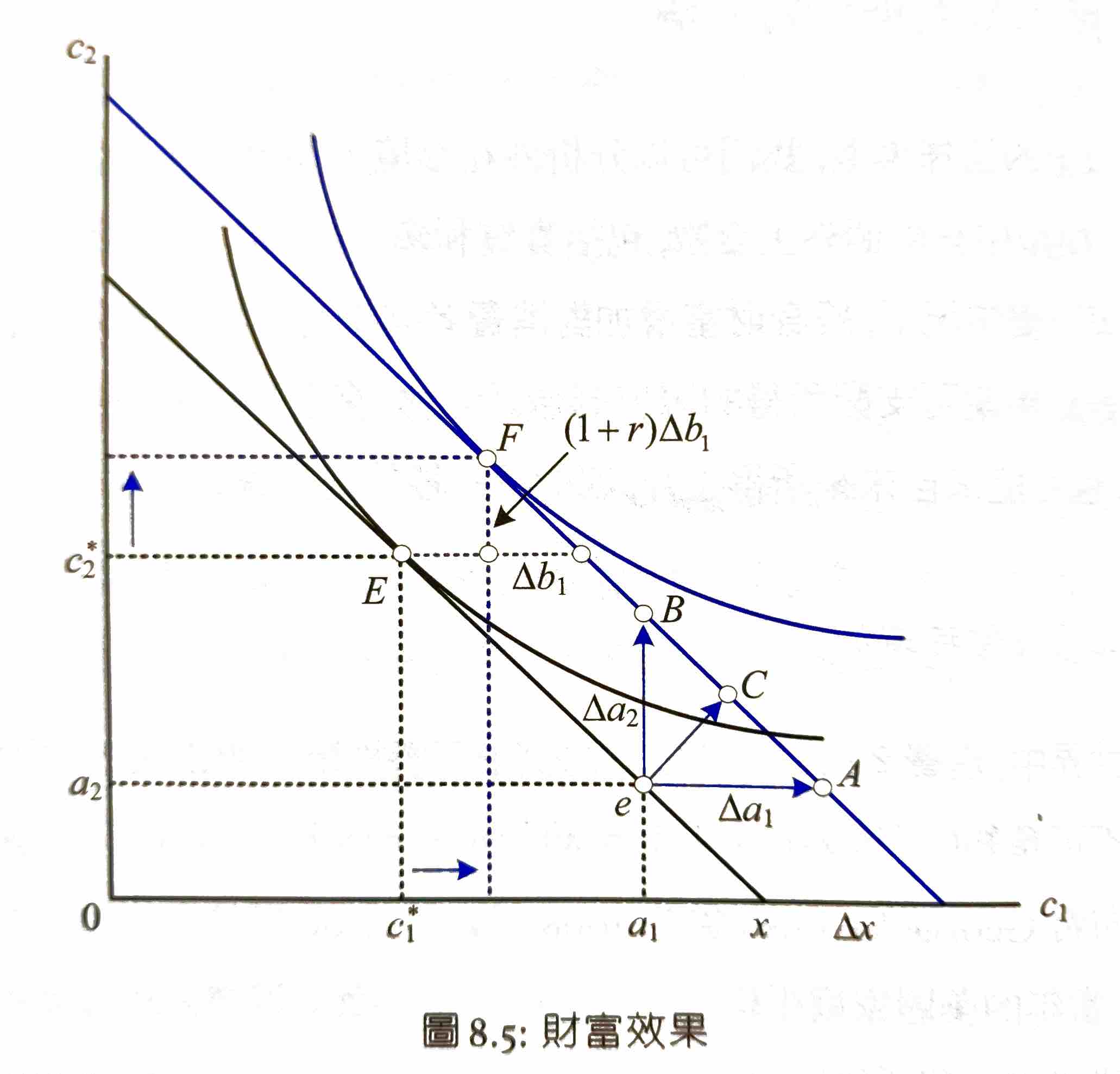
- 本期可支配所得上升,未來不變 → lifetime wealth 上升 → 兩期消費同時增加
- wealth effect
- lifetime wealth 增加量 = 向右平移量 = 向上平移量 / (1+r)
- E → 水平往右 → 延著 new budget line 上升到 F
- 儲蓄增加 \(\Delta b_1\) → \(c_2\) 增加 \((1+r)\Delta b_1\)
- 把今天增加的所得挪到兩期 → 消費平滑
- 本期可支配所得上升,未來不變 → lifetime wealth 上升 → 兩期消費同時增加
- 未來可支配所得增加 (預期)
- lifetime wealth 增加量 = 向上平移量 / (1+r) = 向右平移量
- E → 垂直往上 → 延著 new budget line 下滑到 F
- 儲蓄減少 \(\Delta b_1\)
- 兩期所得等幅增加
- E 直接移到 F
- 儲蓄不變
- 邊際消費&儲蓄傾向
- 邊際消費傾向 MPC, marginal propensity to consume
- 1st 期可支配所得增加 \(\Delta a_1\) → \(MPC=\dfrac{\Delta c_1}{\Delta a_1}\)
- 邊際儲蓄傾向 MPS, marginal propensity to save
- \(MPS=\dfrac{\Delta s_1}{\Delta a_1}=\dfrac{\Delta a_1-\Delta c_1}{\Delta a_1}=1-MPC\)
- 所得變動永久 → MPC=1, MPS=0
- 拿多少就用多少
- 所得變動非永久 → MPC<1
- 分散消費到他期
- 無限多期 → MPC 無限小
- 世代家庭
- 邊際消費傾向 MPC, marginal propensity to consume
- 凱因斯消費函數
- \(C_t=a+bY_t\)
- \(a>0\) = 最低生活水準
- \(0<b<1\) = 邊際消費傾向
- \(C_t\) = t 期消費
- \(Y_t\) = t 期可支配所得
- liquidity 受限 → 沒有 lifetime wealth
- 金融體系不完備,缺乏借貸工具 → 無法透過信用市場移轉各期所得
- \(C_t=a+bY_t\)
(跨期) substitution
- intertemporal substitution effect
- interest rate 上升
- 利率改變後 lifetime wealth 降低,但 utility 不一定
- E 點為原利率的消費點
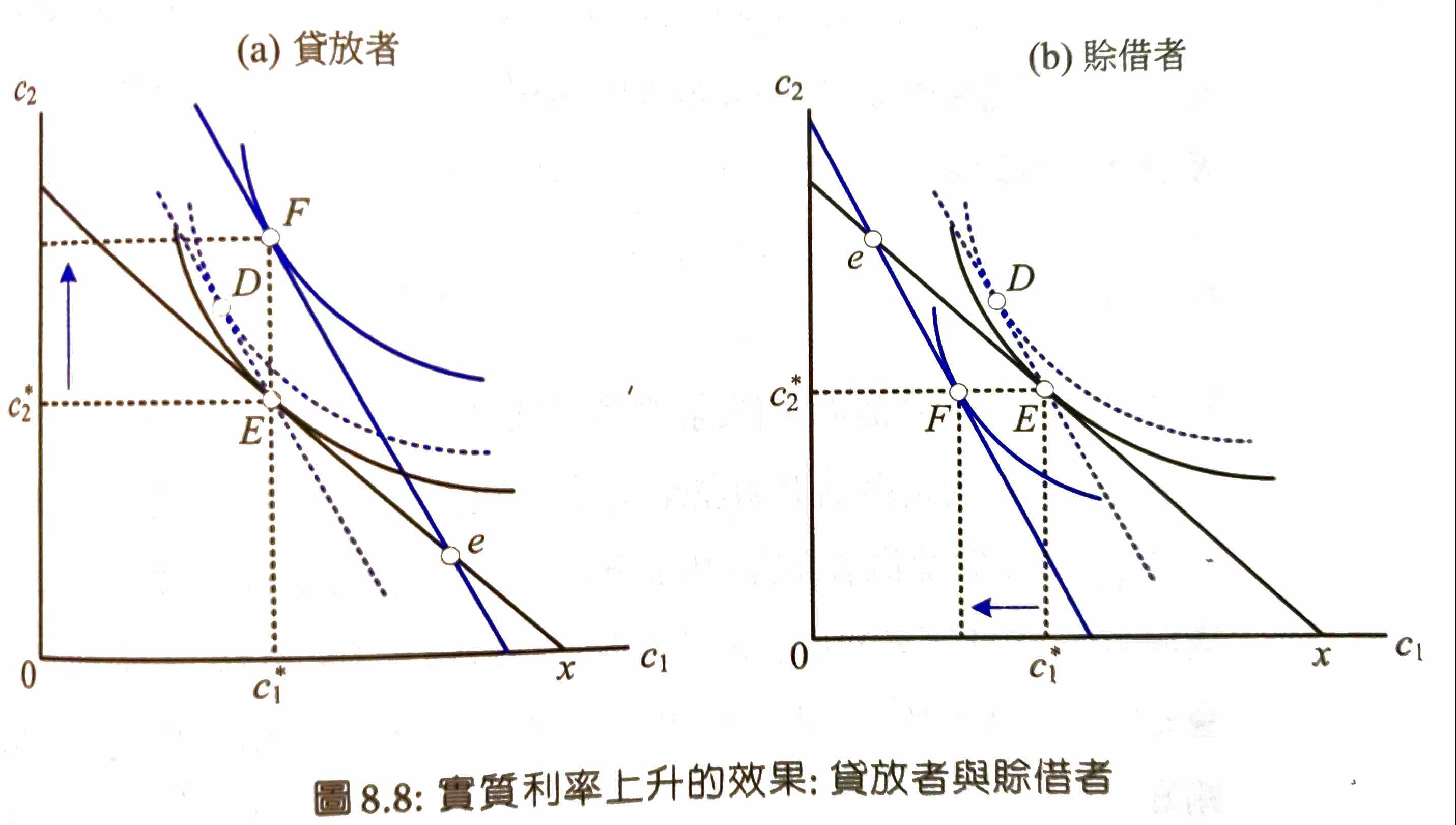
- 貸放者 if endowment e 在 E 右邊 i.e. b1 = a1-c1 > 0
- 利率上升使下期利息所得上升
- 利率上升後的最佳選擇點 utility 較高
- substitution effect → E to D,c1 下降,b1 & c2 上升
- 財富效果 → D to F,c1 & c2 上升
- c2 必然上升,c1 不一定
- 賒借者 if endowment e 在 E 左邊 i.e. b1 = a1-c1 < 0
- 利率上升使下期利息支出上升
- 利率改變後的最佳選擇點 utility 較低
- substitution effect → E to D,c1 下降,b1 & c2 上升
- 財富效果 → D to F,c1 & c2 下降
- c1 必然上升,c2 不一定
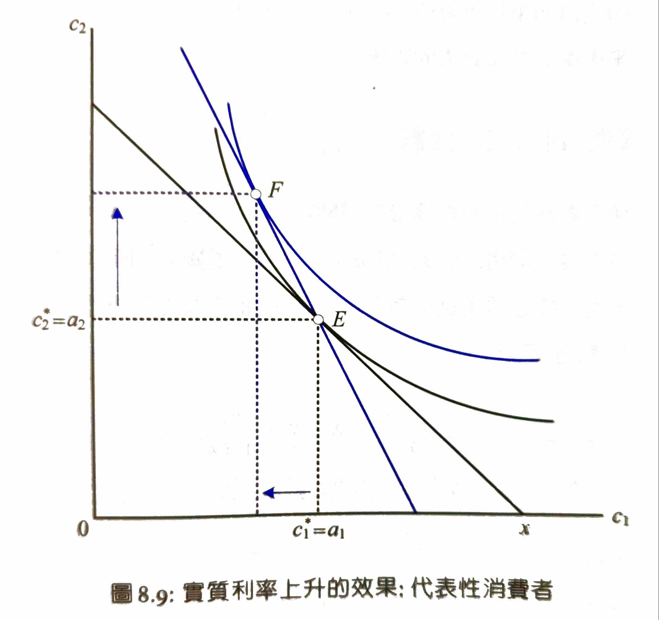
- 代表性消費者 if b1 = 0
- endowment 就在 E,so 只有 substitution effect
- c1 下降,c2 上升
example
設 \(u(c)=lnc\)
- \(u'(c)=\dfrac{1}{c}\)
- \(c_2=\beta(1+r)c_1\)
- \(c_1(1+\beta)=x\)
- \(c_1=\dfrac{x}{1+\beta}=\dfrac{1+\rho}{2+\rho}\left(a_1+\dfrac{a_2}{1+r}\right)\)
- \(s_1=b_1-b_0=b_1=a_1-c_1=\dfrac{1+\rho}{2+\rho}\left(\dfrac{a_1}{1+\rho}-\dfrac{a_2}{1+r}\right)\)
- \(a_1\) 增加
- MPS = \(\dfrac{\Delta s_1}{\Delta a_1}=\dfrac{1}{2+\rho}\)
- MPC = \(\dfrac{\Delta c_1}{\Delta a_1}\) = 1 - MPS = \(\dfrac{1+\rho}{2+\rho}\)
- \(a_1\) & \(a_2\) 等幅增加,設 \(r=\rho\)
- \(s_1\) 不變
- so MPS = 0,MPC = 1
- permanent income = \(c_1=c_2=\dfrac{x}{1+\beta}=\left(\dfrac{1+\rho}{2+\rho}\right)x=\left(\dfrac{1+r}{2+r}\right)x\)
- r 上升
- 設 \(a_1,a_2>0\)
- 跨期替代彈性 intertemporal elasticity of substitution
- \(\dfrac{d\ln(c_2/c_1)}{d\ln MRS_{12}}\)
- \(\ln\dfrac{c_2}{c_1}=\ln\beta+\ln(1+r)\approx\ln\beta+r\)
- r 上升 → c2/c1 必上升
- 消費成長率 g
- \(\ln c_2-\ln c_1 =\ln\dfrac{c_2}{c_1}=\ln(1+g)\approx g\)
- r 上升 x % → g 上升 x%
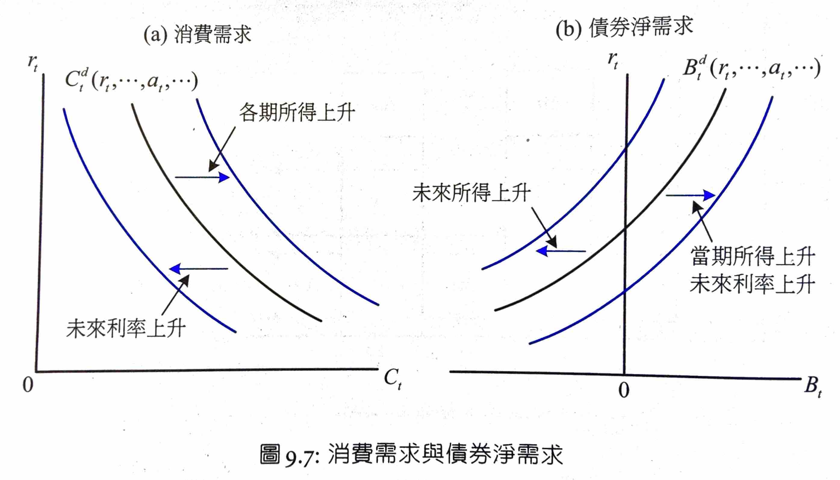
- 消費 & 債券 demand curve
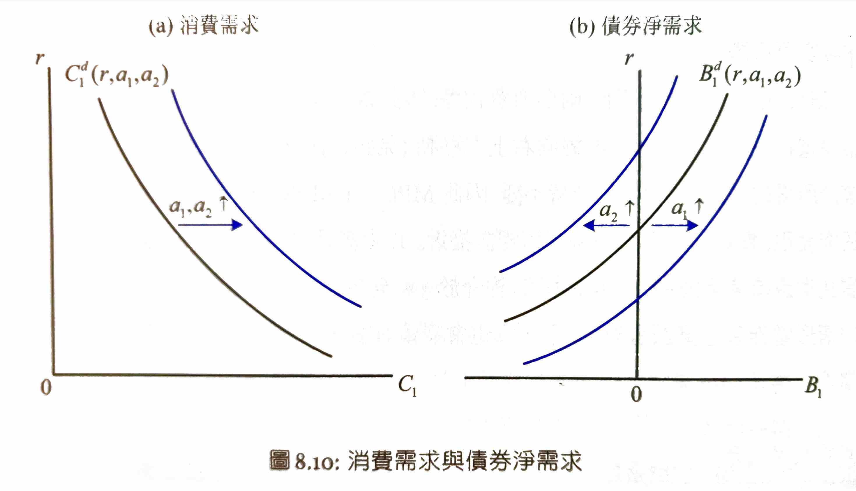
- c1 increase when
- r decrease
- a1 increase
- a2 increase
- b1 increase when
- r increase
- a1 increase
- a2 decrease
- c1 increase when
Ch9 世代家庭的消費與儲蓄
世代家庭決策模型
Also see International Finance#Infinite Horizon Intertemporal Current Account Model
budget constraint
- 儲蓄 = 可支配所得 - 消費支出 = 期末 - 期初債券餘額
- \(c_1+b_1=a_1\)
- \(c_2+b_2=a_2+(1+r)b_1\)
- \(c_3+b_3=a_3+(1+r)b_2\)
- \(c_1+\dfrac{c_2}{1+r}+\dfrac{b_2}{1+r}=a_1+\dfrac{a_2}{1+r}\)
- \(b_2=\dfrac{c_3+b_3-a_3}{1+r}\)
- \(c_1+\dfrac{c_2}{1+r}+\dfrac{c_3}{(1+r)^2}+\dfrac{b_3}{(1+r)^2}=a_1+\dfrac{a_2}{1+r}+\dfrac{a_3}{(1+r)^2}\)
- lifetime wealth = 各期消費 & 最終債券餘額折現值
- \(b_T=0\) if T is not infinite
- \(lim_{T\rightarrow \infty}\dfrac{b_T}{(1+r)^{T-1}}=0\)
- 不一定要 \(b_T\geq 0\)
- as long as \(b_T\) = constant, it's satisfied
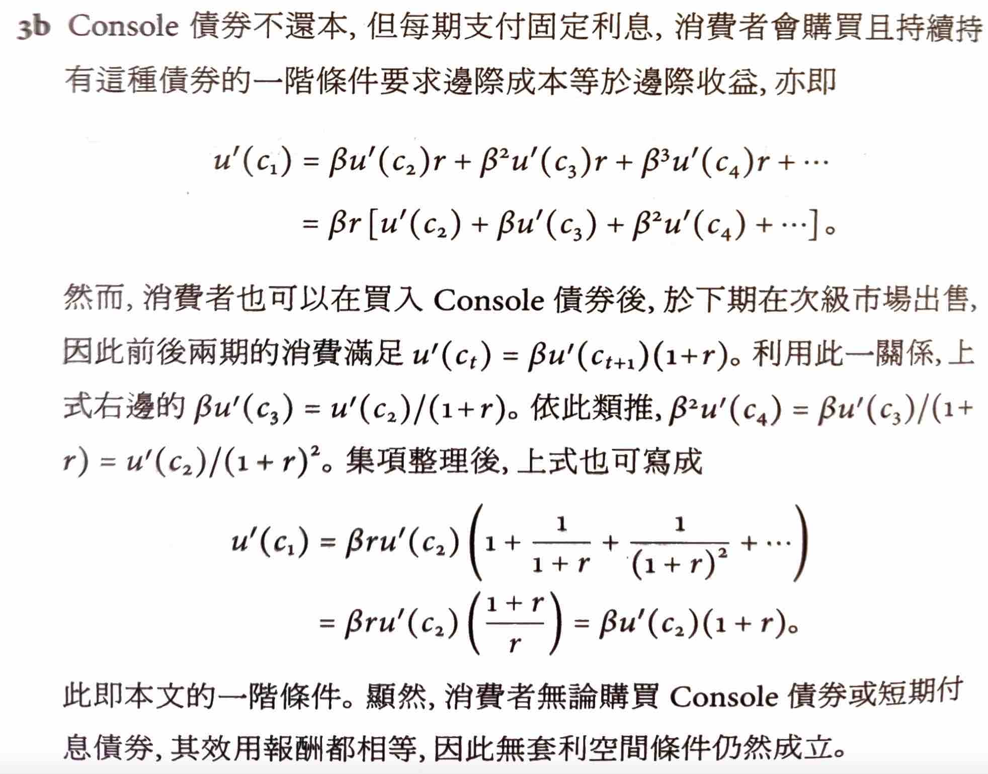
- 無限期債券(只給利息,永遠不還本金)符合條件
- called transversality condition
lifetime wealth
choice
lifetime utility = 各期 utility 折現加總
generalization: same choice for any t
marginal cost of savings (\(c_t\) decrease) = marginal revenue of savings (\(c_{t+1}\) increase)
- \(u'(c_t)=\beta u'(c_{t+1})(1+r_t)\)
- \(u'(c_{t+1})=\beta u'(c_{t+2})(1+r_{t+1})\)
- \(u'(c_t)=\beta^2 u'(c_{t+2})(1+r_t)(1+r_{t+1})\)
任兩期消費的替代關係
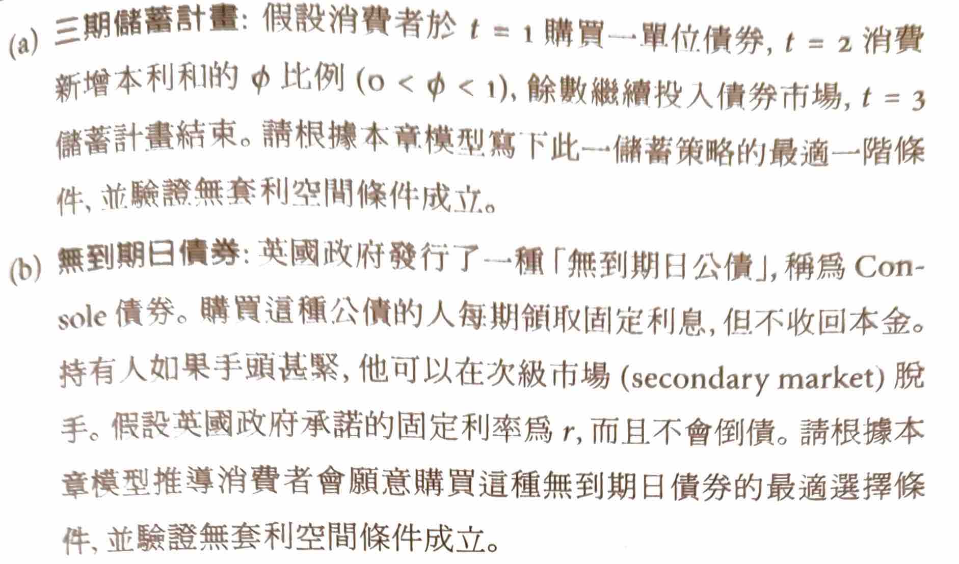
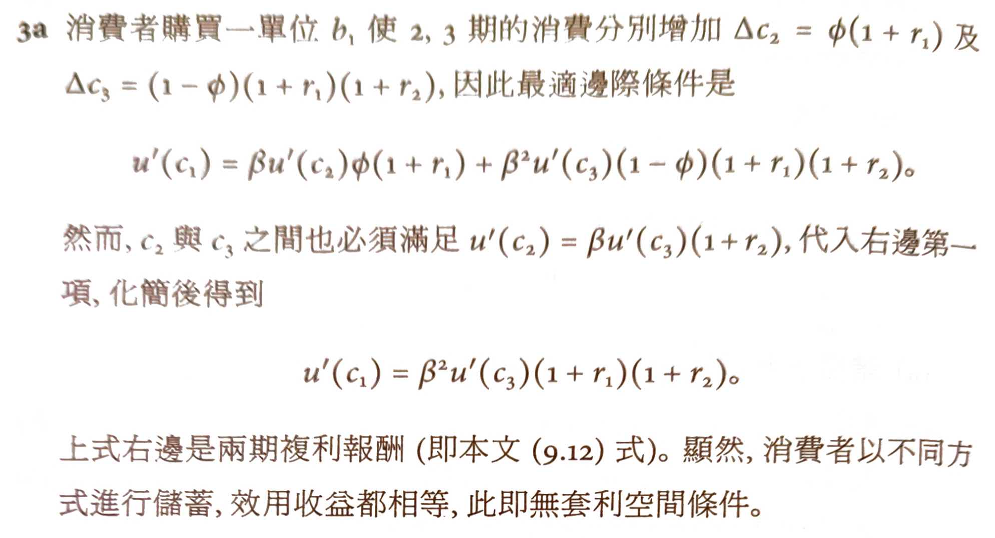
無套利空間條件 (max lifetime utility)
scenario: t 期 save 1, t+1 期 consume partial saving \(r_t\), t+2 期 consume all saving \(1+r_{t+1}\)
又
so
跨期消費型態
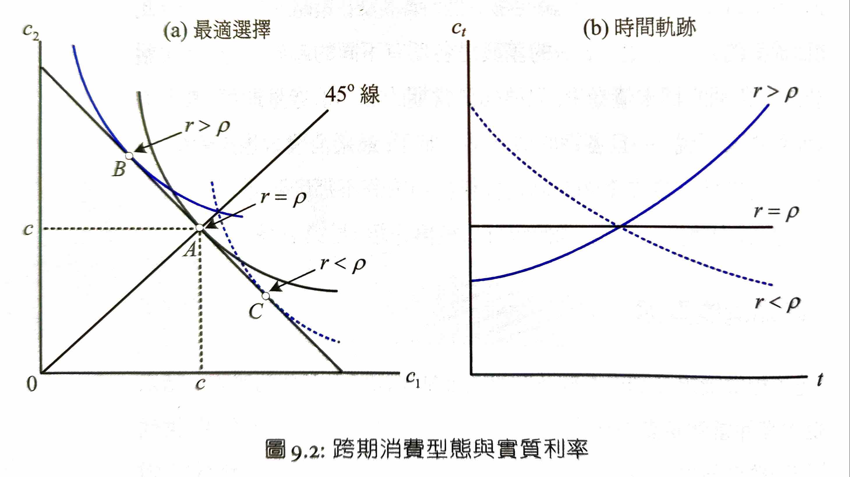
see #費雪兩期模型#utlity
If \(r=\rho\), the marginal utility of consumption is the same in every period
If \(r>\rho\), \(u'(c_{t})>u'(c_{t+1})\), so \(c_{t} < c_{t+1}\) at max utility point
If \(r<\rho\), \(u'(c_{t})<u'(c_{t+1})\), so \(c_{t} > c_{t+1}\) at max utility point
Assume \(u(c)=\ln{c}\)
消費成長率 = interest rate - time preference factor
Scenario
As 9.3(a), the expected interest rate will increase in t=10~20 and then drop back down
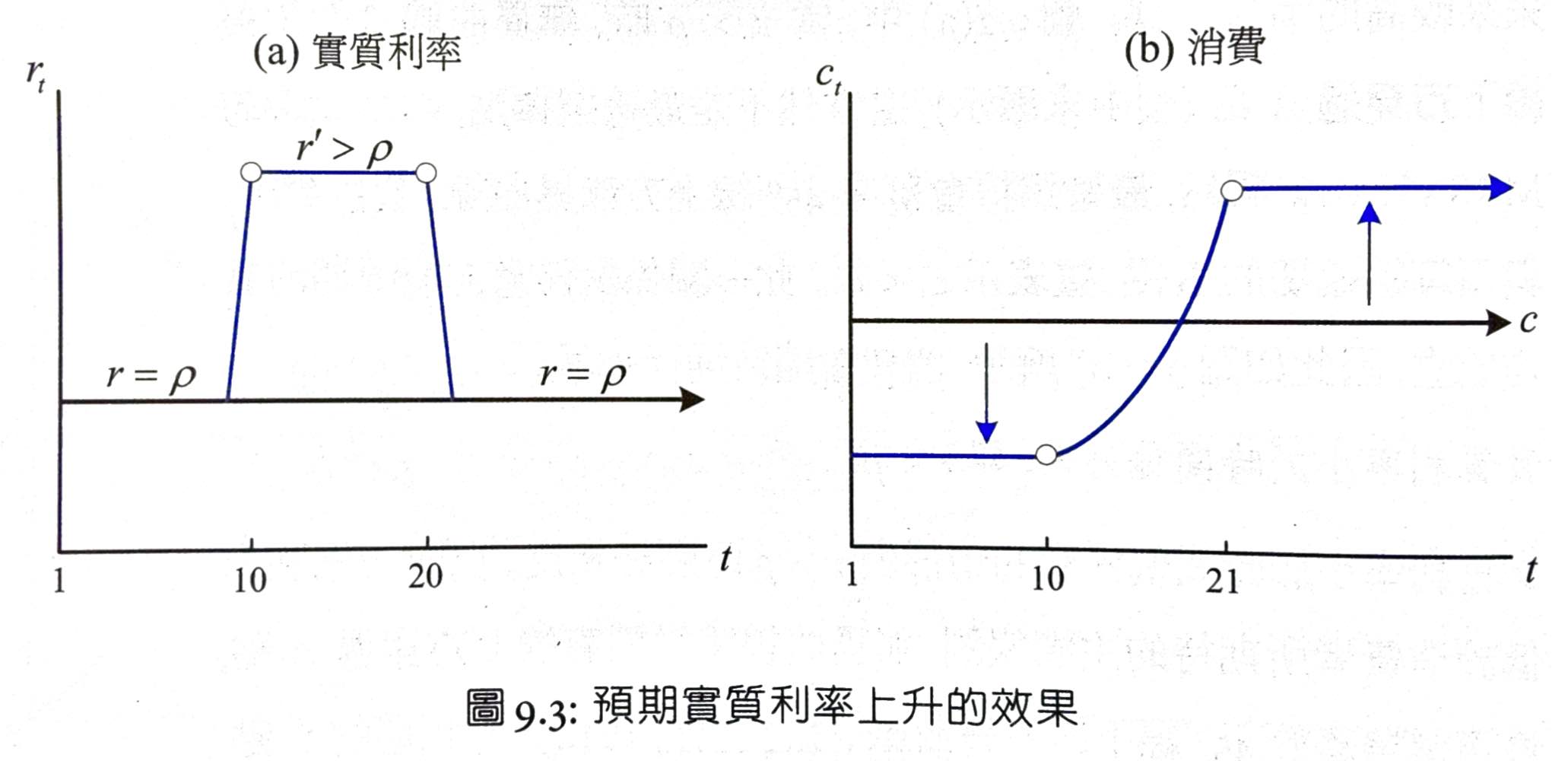
- At t=1~10, the consumer decreases its consumption to a lower constant
- At t=10-20, since \(r-\rho>0\), 消費成長率為正, so consumption increases in each period
- At t=20-30, consumption stays as a high constant
The change of interest rate will also trigger income effect, up or down shifting the overall curve depending on if the consumer has a positive or negative wealth.
恆常所得假說 permanent income
income = permanent income + transitory income
- \(y\) = total oncome
- \(y^P\) = 恆常所得 permanent income
- \(y^T\) = 暫時所得 transitory income
而 consumption 並非取決於 total income,而是 permanent income
\(\phi\) = constant, normally close to 1. When \(\phi=1\), a consumer spends all permanent income and save all transitory income
In 兩期模型,permanant income \(\bar{y}\) = where \(c_1=c_2\) (B 點)
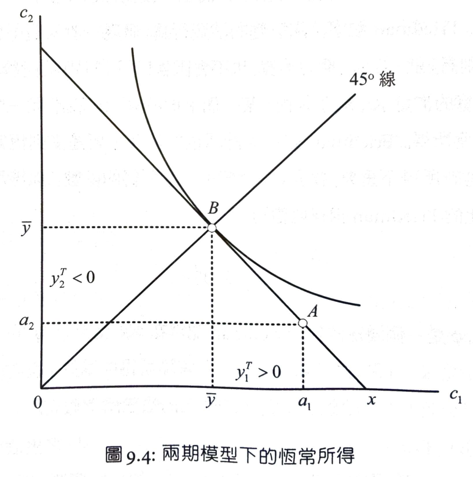
A 點為實際所得
When \(r=\rho\), utility function 切 budge constraint at B, \(c_1=c_2\), \(s_1=y_1^T=a_1-\bar{y}\)
無限期
\(x_t\) = t 期開始的終身財富 = 各期 permanent income 折現總值
intuition: 把 \(x_t\) 存到銀行,每個月得到的利息折現值 = 該期 permanent income
Recursion betwen \(x_t\) & \(x_{t+1}\)
Now we find the recursive relationship between each period of lifetime wealth \(x\). Assume we come in with no initial bonds \(b_0\):
\(b_1=a_1-c_1\)
intuition: pretty straightforward, save all you've left in this period
If \(r=\rho\), then the consumption in each period is the same
Finding \(\phi\)
assume \(u(c)=\ln{c}\) and \(r\) may != \(\rho\)
\(\phi=1\) when \(r=\rho\)
the growth rate of lifetime wealth, consumption & permanent income = \(\dfrac{1+r}{1+\rho}\)
所得變動影響
Assume \(r=\rho\)
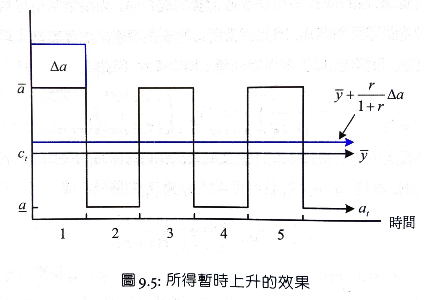
MPC = \(\dfrac{\Delta c_1}{\Delta a_1}=\dfrac{r}{1+r}\approx 0\)
MPS = \(\dfrac{\Delta s_1}{\Delta a_1}=\) 1 - MPC \(=\dfrac{1}{1+r}\approx 1\)
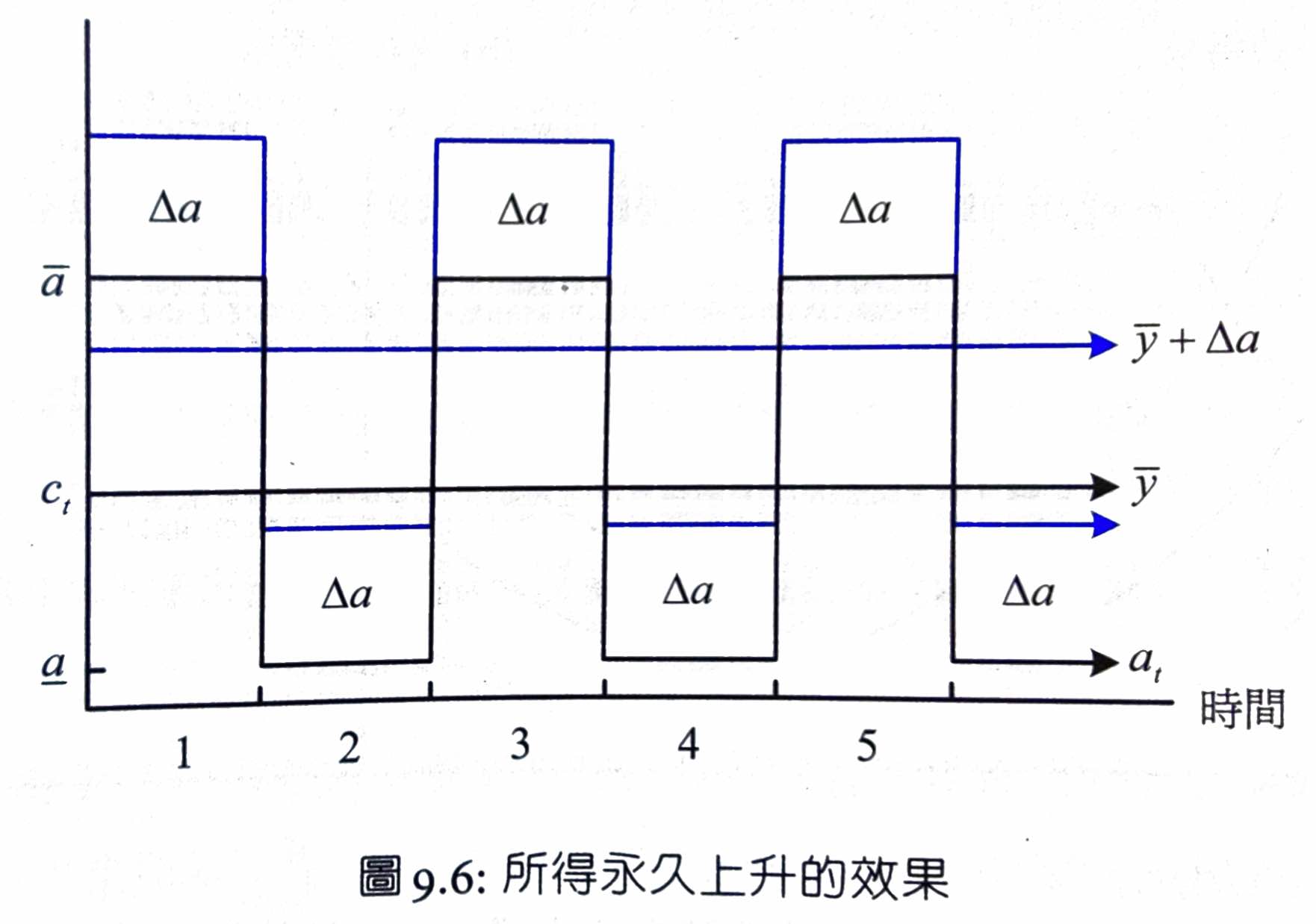
MPC = \(\dfrac{\Delta c_1}{\Delta a_1}=1\)
MPS = \(\dfrac{\Delta s_1}{\Delta a_1}=\) 1 - MPC \(=0\)
直接把多的錢消費掉
consumption & bonds
Problems
Ch10 Endowment Economy Equilibrium Analysis
endowment economy: no production, only endowment in each period
Endowment Economy 全面均衡
政府用 bonds 貼赤字
- \(G\) = government purchase
- \(B^g\) = government bonds
- \(r\) = bond interest rate
- \(T\) = tax
budget deficit \(D\) = expenditure - tax
t 期折現 factor \(q_t=\prod_{i=1}^{t-1}(\dfrac{1}{1+r_i})\)
均衡條件
商品市場
bonds market (d = demand)
- \(T_t=G_t+(1+r_{t-1})B^g_{t-1}-B^g_t\)
- \(C^d_t+B^d_t=(Y_t-T_t)+(1+r_{t-1})B_{t-1}\)
- \(C^d_t-Y_t+T_t+B^d_t=(1+r_{t-1})B_{t-1}\)
since 流通 bonds = 政府發行 bonds
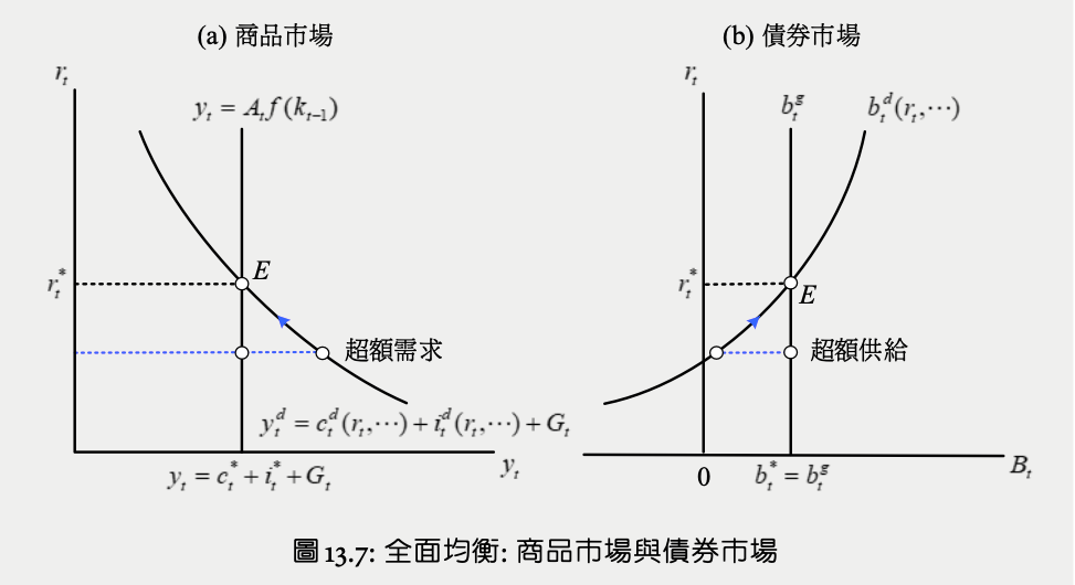
So 商品市場超額需求 + 債券市場超額需求 = 0
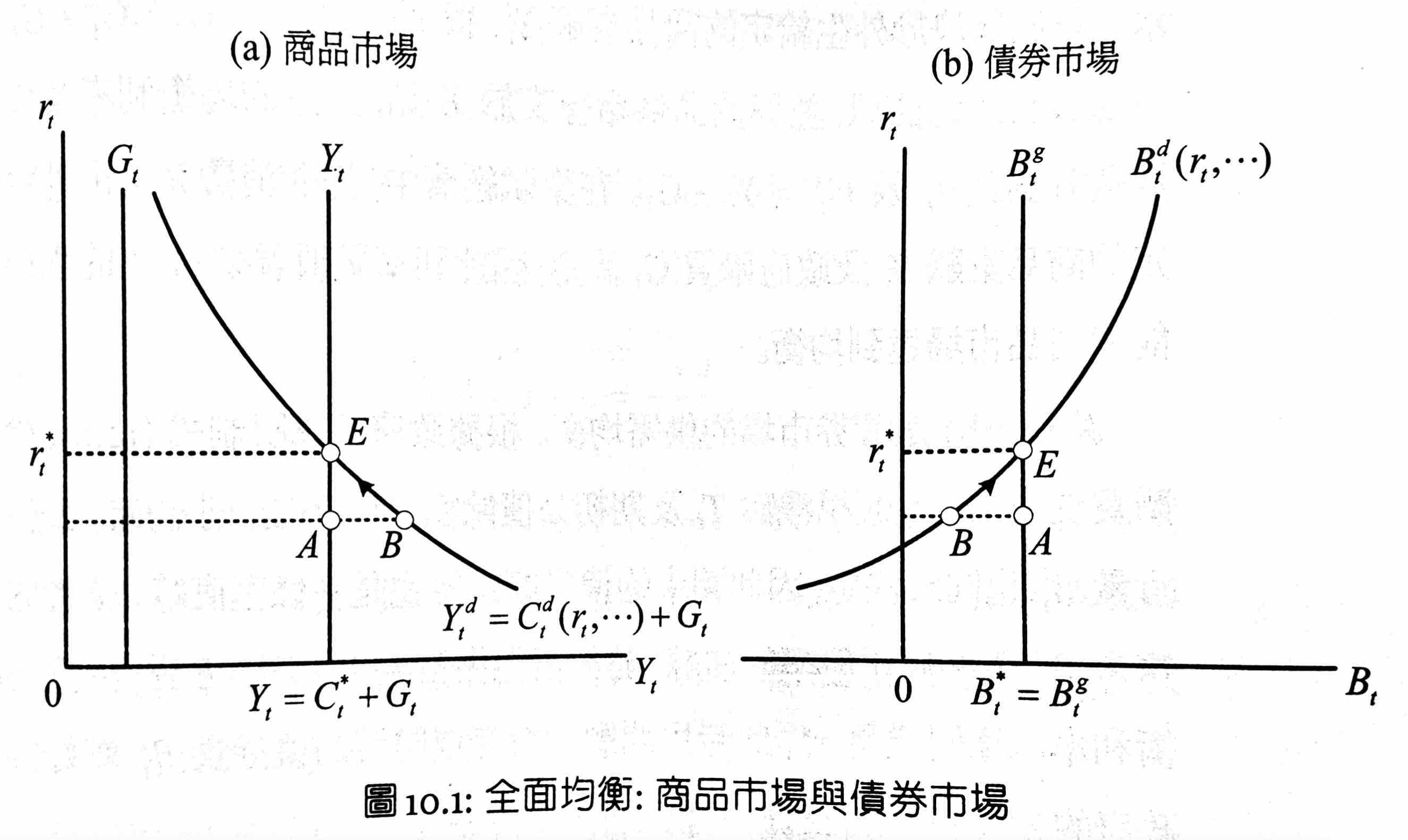
\(Y_t\) & \(G_t\) are given (exogenous). Reach equilibrium at \(r=r^*\)
\(r<r^*\) -> consumption demand > income -> sell bonds to raise money -> bonds supply > demand -> interest rate rises to attract bonds buyer
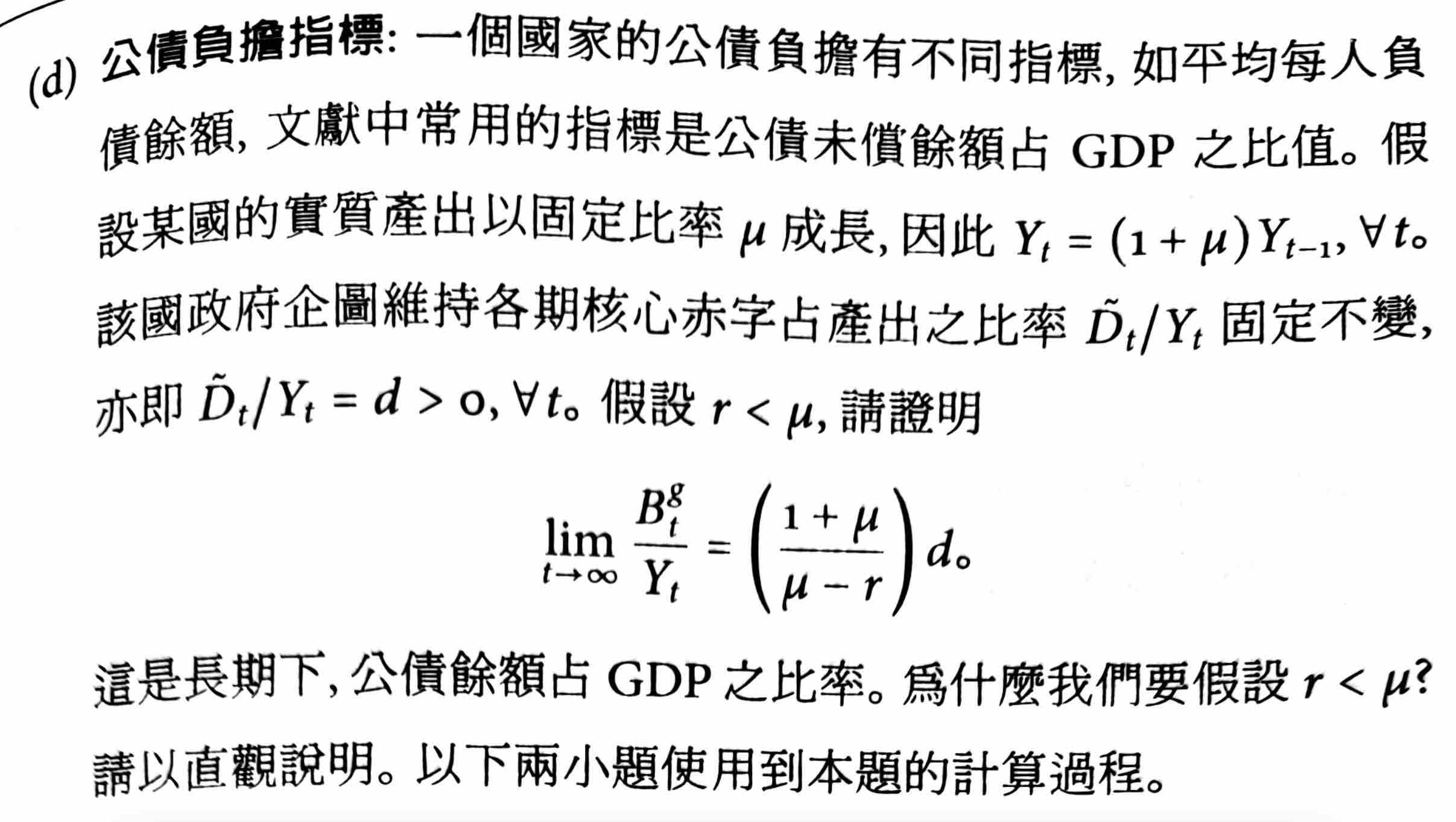
Equilibrium interest rate & growth of income
Assume the growth rate of \(Y_t\) = \(\mu\)
Assume \(G_t=0\). Since \(C_t=Y_t-G_t=Y_t\), the growth rate of \(C_t\) is \(\mu\) as well
Assume \(u(C_t)=\ln C_t\)
So the higher the \(\mu\), the higher the \(r\)
We can also get this from graphical analysis
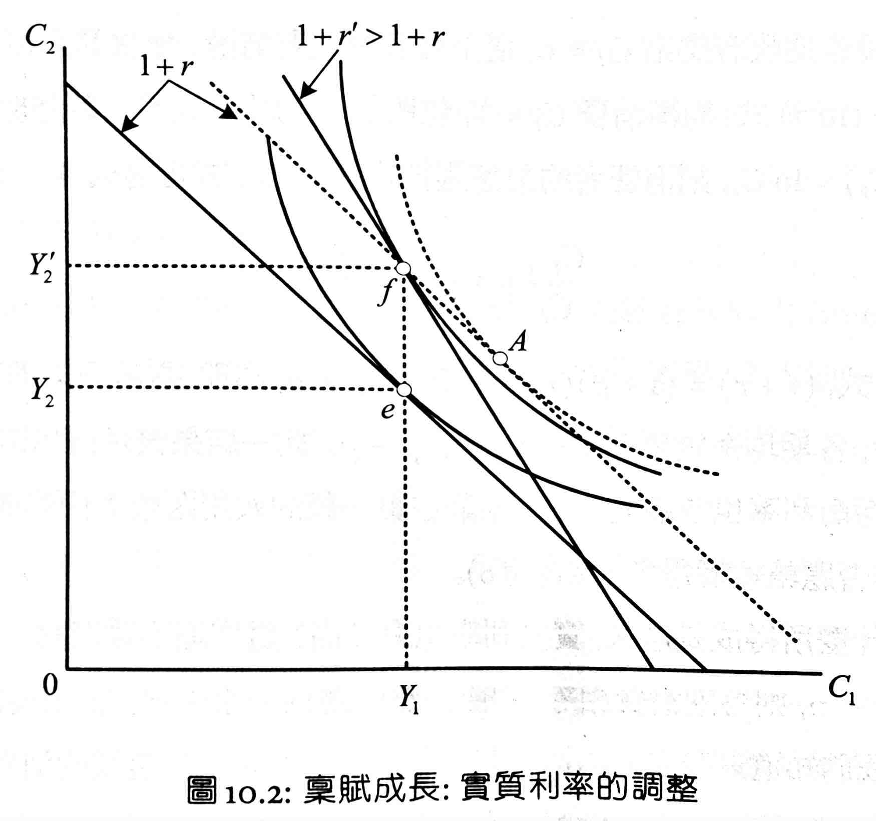
Original endowment is e. Now \(Y_2\) rises to \(Y_2'\). Since \(r\) isn't changed, the budget constraint simply up shifts, resulting in a new equilibrium point A.
In A, \(C^d_1>Y_1\) -> 超額需求 in 商品市場 -> 超額供給 in 債券市場 -> interest rate rises -> budge constraint slope increases -> new equilibrium point f
Conclusion: 成長快的國家 利率應較高
In real life
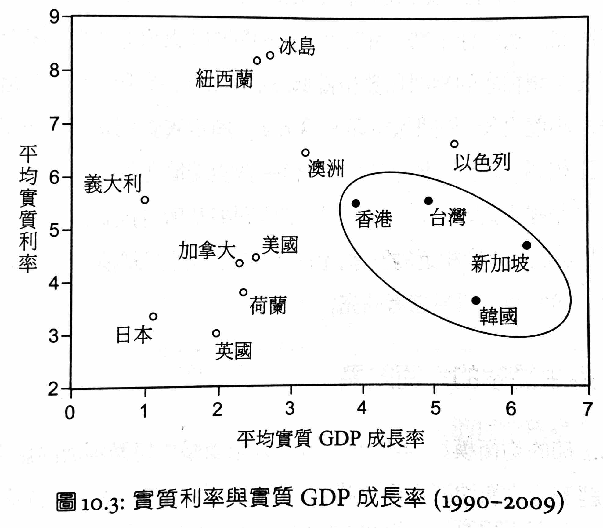
correlation efficient = 0.08, or 0.44 if excluding 亞洲四小龍
deficit & GDP growth rate & interest rate

外生衝擊均衡效果
endowment temporarily decreases
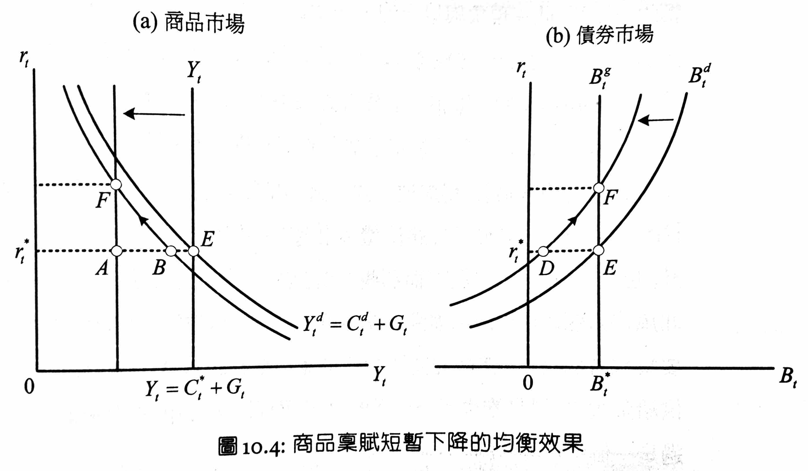
- 商品市場超額需求
- 債券市場超額供給
- sell bonds to raise money for consumption / decrease savings i.e. buying bonds when income reduced
- interest rate rises
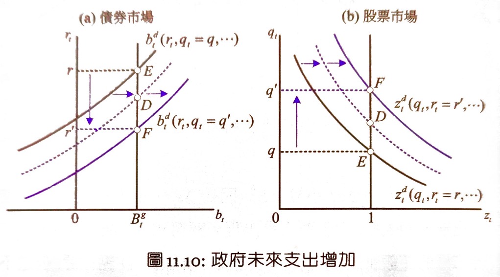
government consumption temporarily increases
The increase of government expenditure has to come from tax or bonds, so either an increase in current tax or in future tax.
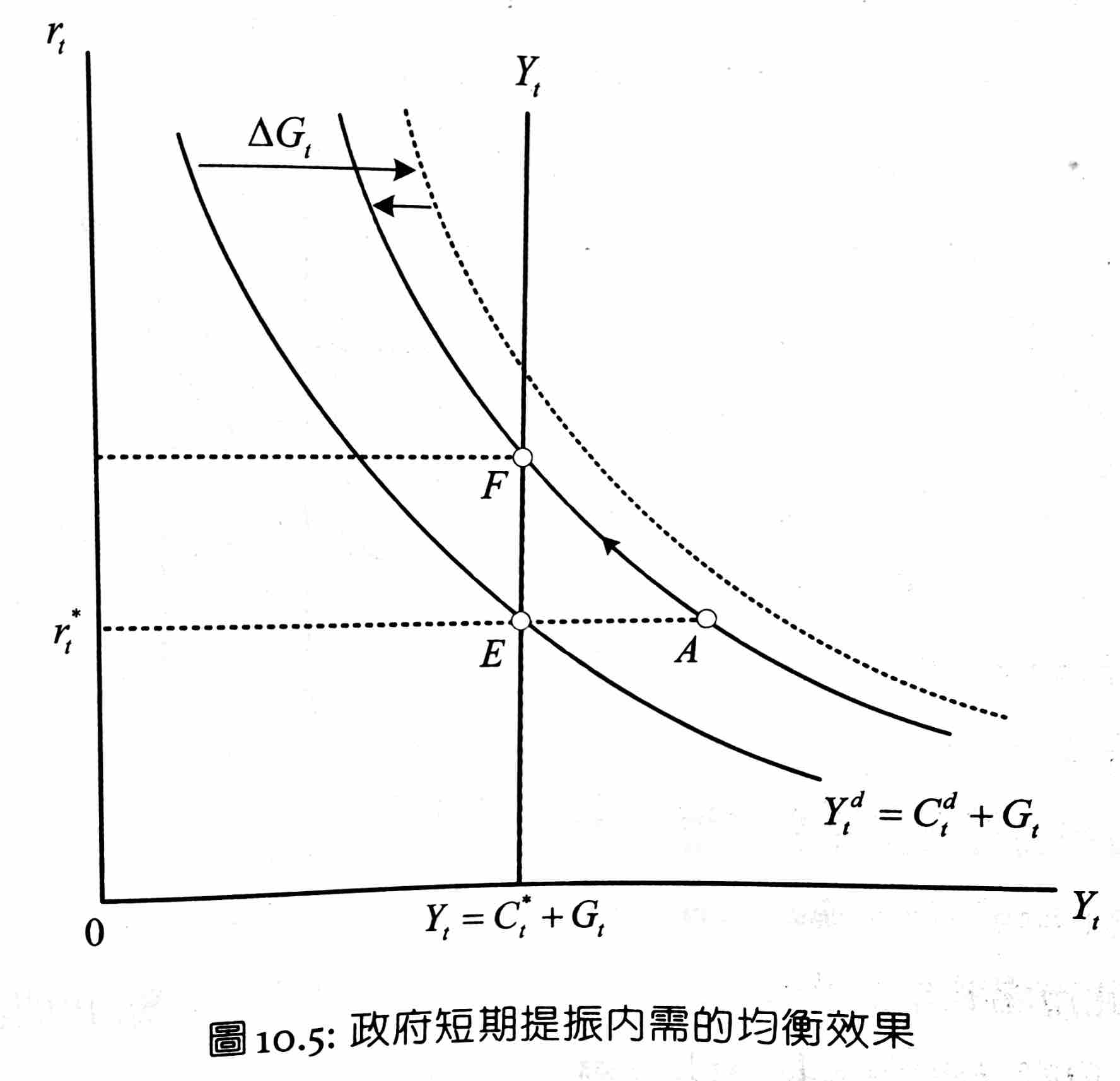
E -> A
- government expenditure increase 直接效果: \(C^d_t\) right shifts to 虛線
- tax increase income effect: \(C^d_t\) left shifts a bit
A -> F
- 商品市場超額需求 -> \(r\) increases -> consumption decreases
For 債券市場
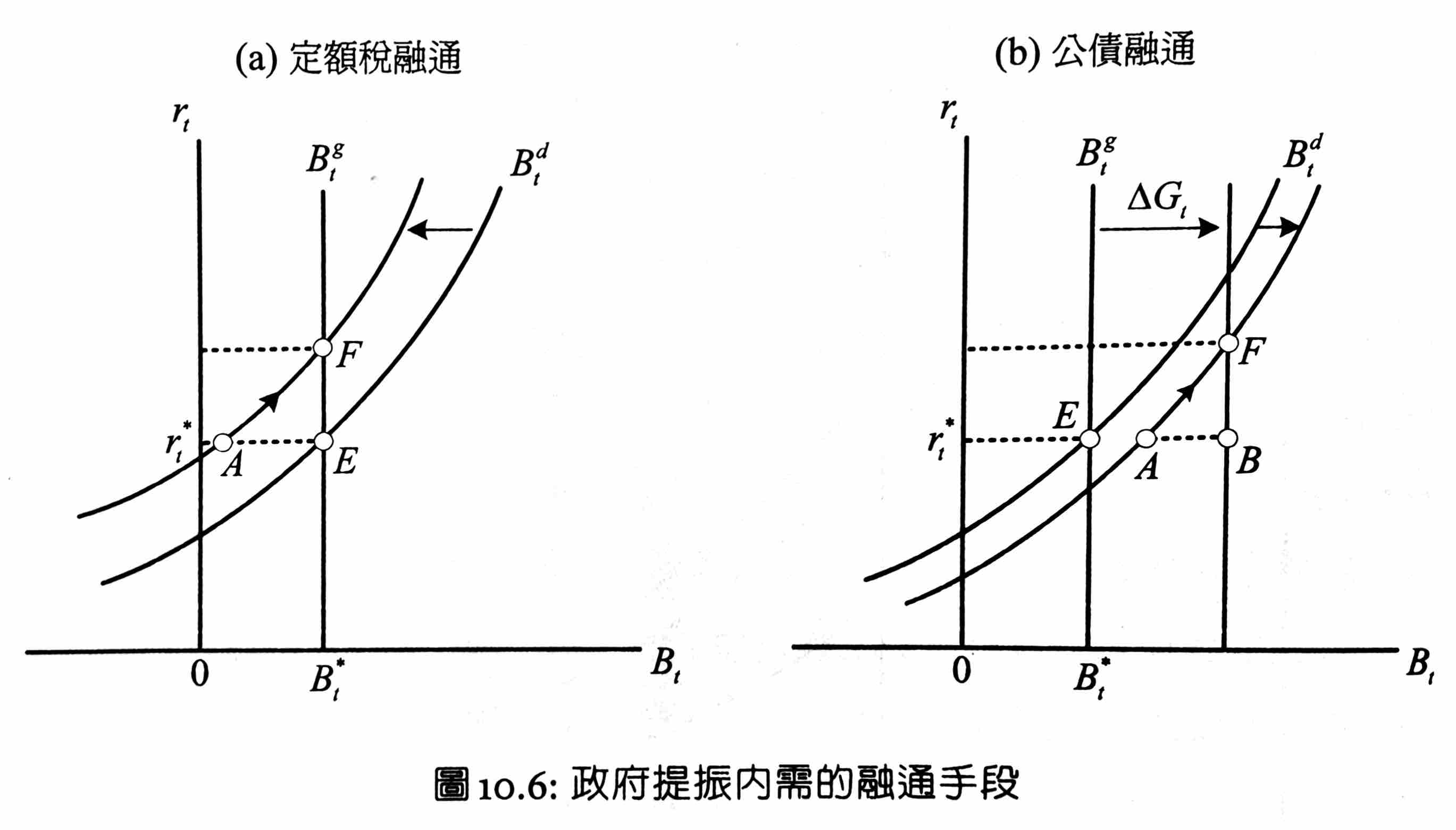
if use 定額稅
- 課稅後所得下降 -> 儲蓄意願下降 -> bonds demand left shifts -> bonds supply > demand -> interest rate increases
if use bonds
- \(B^g_t\) right shifts
- future income decreases due to future tax -> 儲蓄意願上升 -> bonds demand left shifts
- new \(B^g_t\) & \(B^d_t\) intersect at a higher \(r_t\)
- income unchanged -> consumption decrease = saving / bonds increase
- \(\Delta B^d_t = \Delta C^d_t < \Delta G_t = \Delta B^g_t\)
李嘉圖等值論 Ricardian Equivalence Theorem
赤字減稅政策
two-period
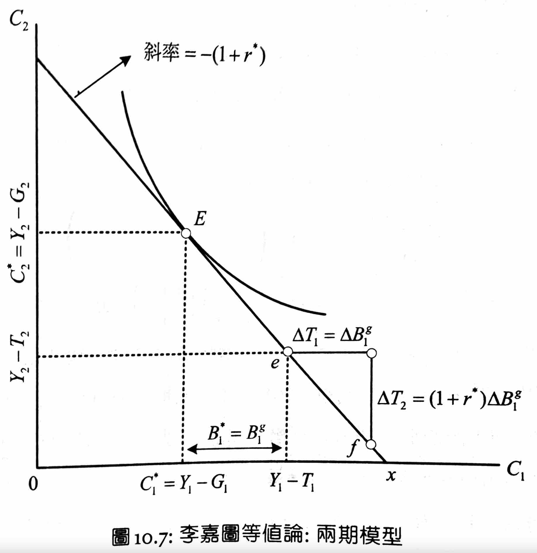
E is optimal point
- \(C_1^*=Y_1-G_1\)
- \(C_2^*=Y_2-G_2\)
- \(r^*\) is equilibrium interest rate
e is the original endowment
- \(C_1=Y_1-T_1\)
- \(C_2=Y_2-T_2\)
f is the endowment after doing 赤字減稅政策 deficit-financed tax cut
- t=1 減稅但多發公債
- \(\Delta T_1=-\Delta B^g_1\)
- \(\Delta T_2=(1+r^*)\Delta B^g_1\)
- \(\Delta \text{lifetime wealth}=-\Delta \text{lifetime tax}=\Delta T_1+\dfrac{\Delta T_2}{1+r^*}=0\)
- E is still the optimal point
infinite horizon
- t=1 少課稅 \(\Delta B^g_1\) 發行 consol (無限期 bond)
- 之後每期多課稅 \(r\Delta B^g_1\) 付息
- \(\Delta \text{lifetime tax}=\sum^\infty_{t=1}\dfrac{\Delta T_t}{(1+r)^{t-1}}=-\Delta B^g_1+\sum^\infty_{t=2}\dfrac{r\Delta B^g_1}{(1+r)^{t-1}}=0\)
What Ricardian doesn't consider
- tax 對於個體的負擔並非均等
- 不同 consumer or 同 consumer 不同世代的 tax 負擔不一樣
- e.g. 學生時期減稅沒差,但長大後增稅卻有差
- though they're averaged out when looking at a grand/macro scope
- 不同 consumer or 同 consumer 不同世代的 tax 負擔不一樣
- 政府減增稅期限可能超過個體生命範圍
- e.g. 將死老人減稅,增稅時已死,所以還是會增加消費
- but 用世代家庭的觀點看,人們會將後代看作自身
- 借貸市場不完全
- 並非所有人都有 full access to the bonds market
- look at a person that is forbidden to borrow money
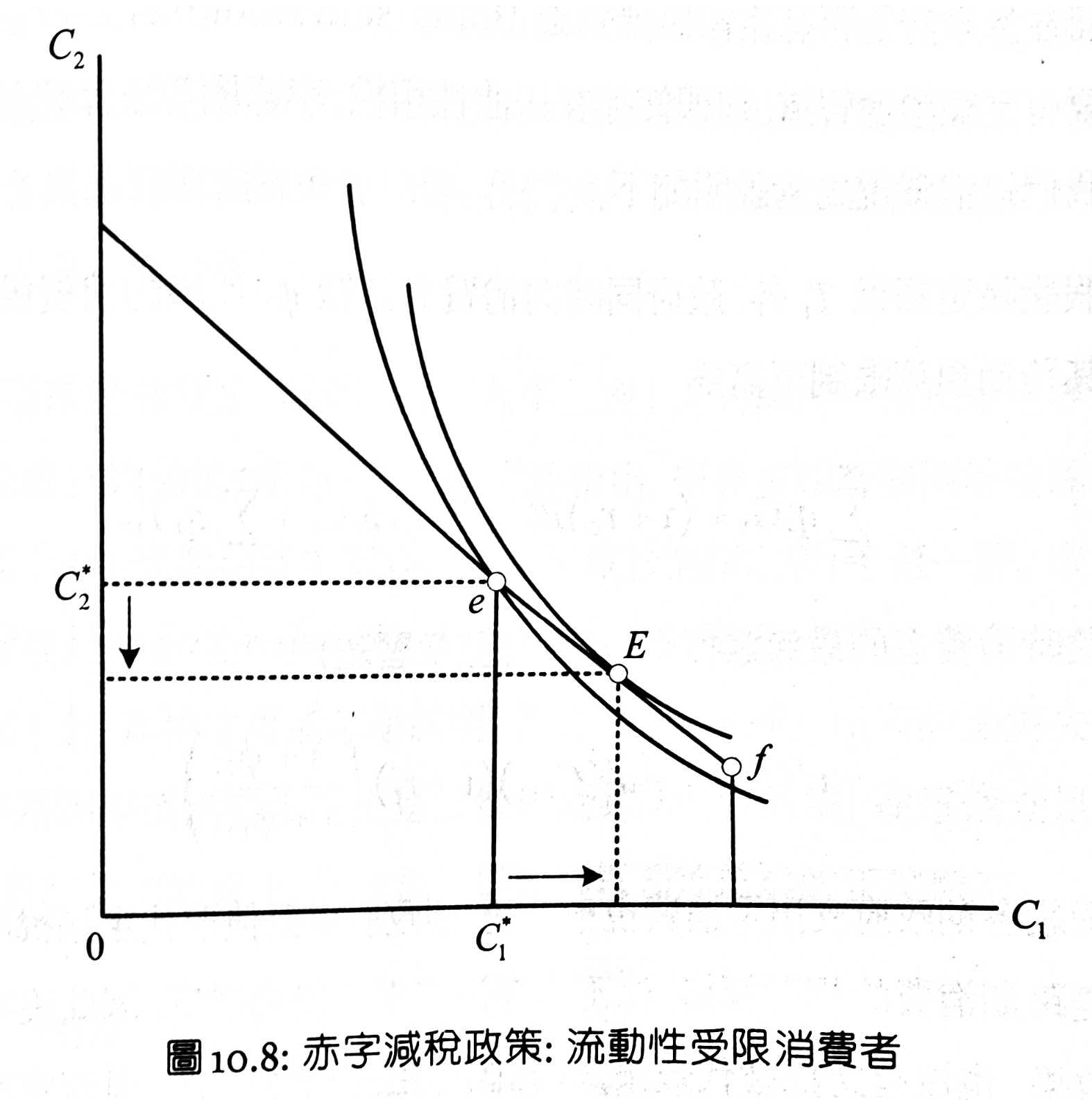
- original endowment = e, since he can't borrow money, his equilibrium point is still e
- endowment after deficit-financed tax cut = f, since he can lend money, his equilibrium point = max utility point = E
- so after applying deficit-financed tax cut, there is an over demand in the consumption market, driving the interest rate up, 排擠他人的 consumption
- other tax methods
- as long as there is 定額通融管道 lump-sum resource,Ricardian is correct even if there is 扭曲性租稅
- assume a \(\phi_t\) consumption tax in addition of lump-sum tax \(T_t\)
- \(\sum^\infty_{t=1}q_tG_t+(1+r_0)B^g_0=\sum_{t=1}^\infty q_t\phi_t+\sum_{t=1}^\infty q_tT_t\)
- government expenditure = tax income
- \(u'(C_t)=\beta u'(C_{t+1})(1+r_t)\left(\dfrac{1+\phi_t}{1+\phi_{t+1}}\right)\)
- using tax to pay for bonds doesn't change anything
- \(\sum^\infty_{t=1}q_tG_t+(1+r_0)B^g_0=\sum_{t=1}^\infty q_t\phi_t+\sum_{t=1}^\infty q_tT_t\)
- but if not use lump-sum tax but consumption tax to pay for bonds
- \(\phi_t\) decreases while \(\phi_{t+1}\) increases -> \(C_t\) increases while \(C_{t+1}\) decreases
- if no bonds & lump-sum tax
- recession -> fiscal deficit -> increase tax rate to pay for it -> further recession
- boom -> fiscal surplus -> decrease tax rate -> further boom
國民年金 National Pension
2 systems
- 隨收隨付 pay-as-you-go PAYG
- 所得重分配
- 對年輕人課稅,轉給老人
- 全額提撥 fully-funded
- forced saving
- for an individual,年輕時與政府共同繳款到帳戶,老了領出來
各國往往 start with fully-funded, but end up hybrid as time goes
pay-as-you-go PAYG
overlapping generations model / consumption loan model
Assume each person lives for 2 periods, with endowment = \(y_1\) when young and \(y_2\) when old.
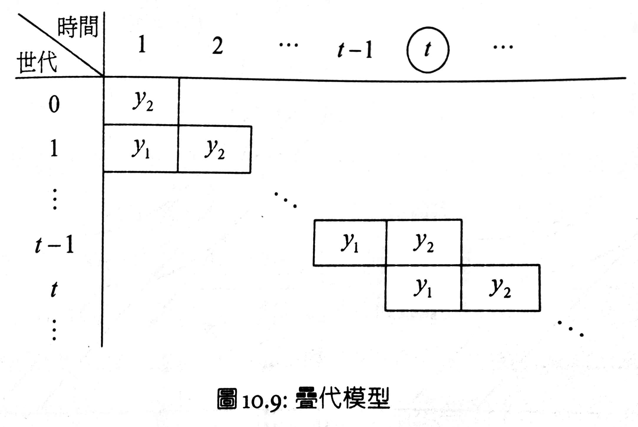
Each period consists of 2 generations, one young another old.
Old people don't have access to loan market as they'll be dead in the next period and unable to pay off loans.
PAYG becomes a way for money flow between the young and the old.
Assume PAYG starts at t=1, giving each old man \(b\)
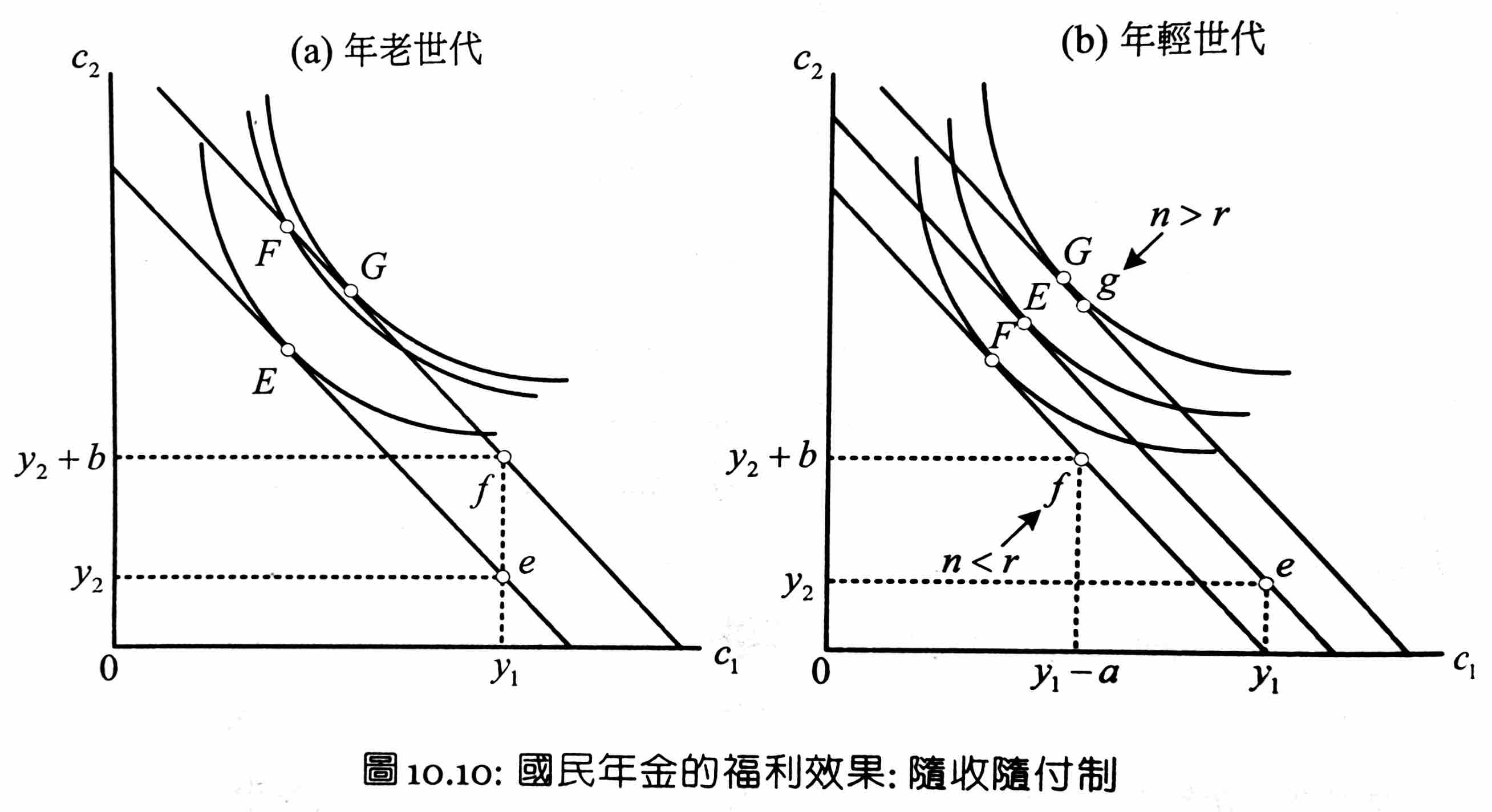
For the old (born in t=0)
- endowment without PAYG = e
- equilibrium point = E
- endowment with PAYG = f
- equilibrium if not knowing PAYG when young = F
- equilibrium if knowing PAYG when young = G
For the young (born in t=1)
- \(N_t\) = num of people borning in t=t
- \(N_t=(1+n)N_{t-1}\) i.e. population growth rate = \(n\)
- each young needs to pay \(a=\dfrac{bN_{0}}{N_1}=\dfrac{b}{1+n}\)
- lifetime wealth = \(c_1+\dfrac{c_2}{1+r}=(y_1-a)+\dfrac{y_2+b}{1+r}=y_1+\dfrac{y_2}{1+r}+\dfrac{(n-r)b}{(1+r)(1+n)}\)
- when \(n>r\) lifetime wealth increases, E -> G
- pareto improvement for the society
- when \(n<r\) lifetime wealth decreases, E -> F
- many developed countries
fully-funded
In a complete market, forced saving is meaningless as you can just go to the market and cancel it out.
Assume all the money comes from yourself and the interest rate is in the national pension account is the same as the market interest rate.
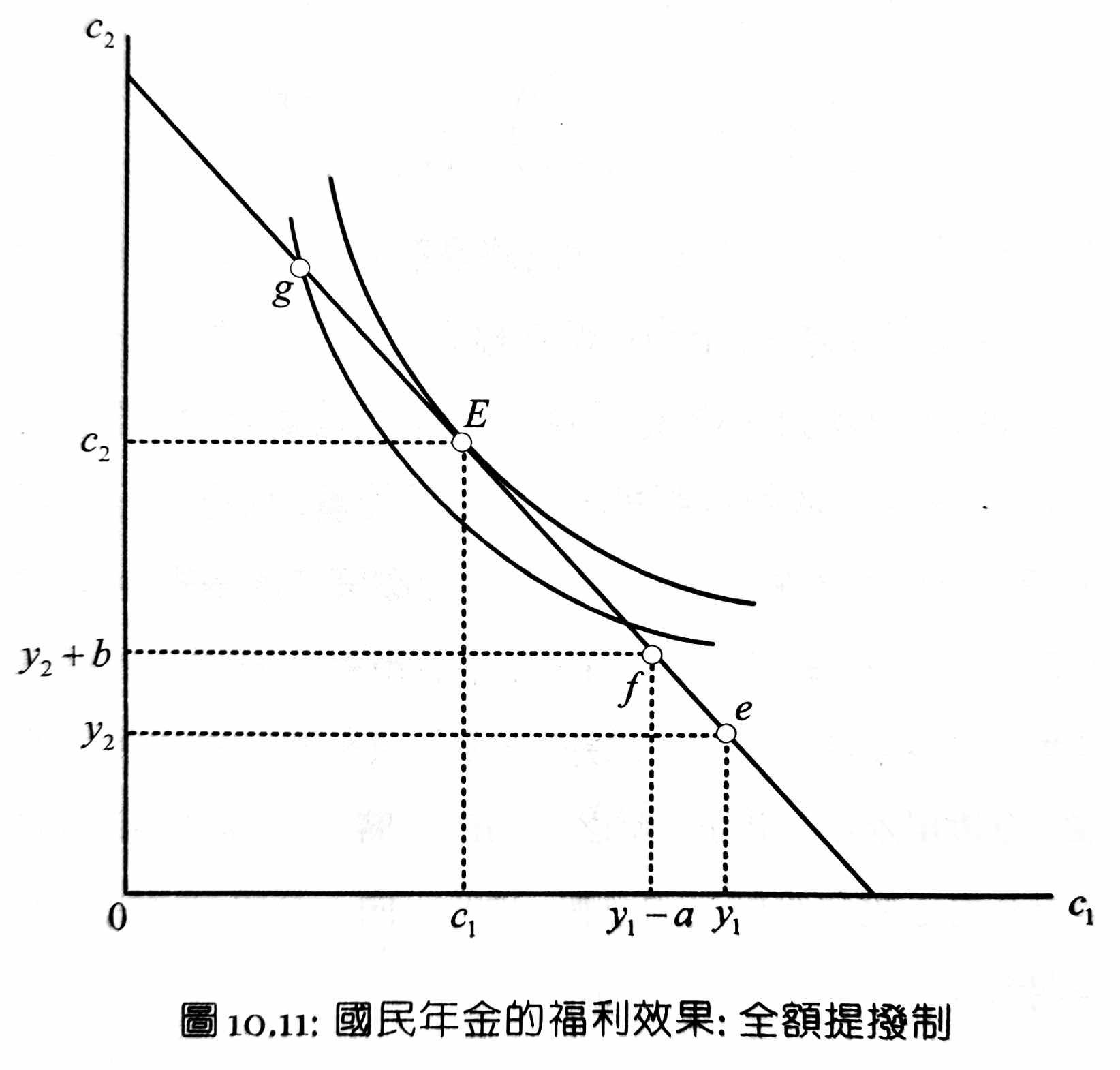
If a person doesn't have access to the loan market and the forced saving > the optimal saving, then he will be stuck in point g, decreasing his utility.
Problems
Problem 10.6
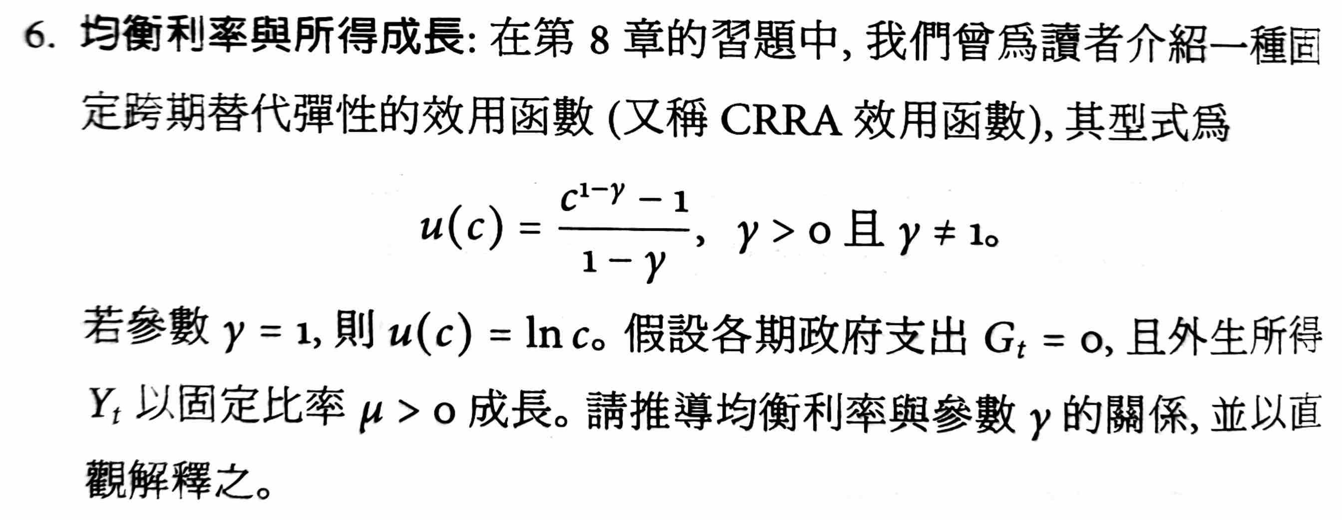
- \(c_2=(1+\mu)c_1\)
- \(u'(c_1)=\beta(1+r)u'(c_2)\)
- \(c_1^{\gamma}=\beta(1+r)c_1^{-\gamma}(1+\mu)^{-\gamma+1}\)
- \(\dfrac{1+r}{1+\rho}=(1+\mu)^{\gamma-1}\)
- \(\ln(1+r)-\ln(1+\rho)=(\gamma-1)\ln(1+\mu)\)
- \(r-\rho\approx(\gamma-1)\mu\)
- \(r=\rho\) when \(\mu=0\) or \(\gamma=1\)
Ch11 資產定價模型
Lucas Tree Model
An endowment society where all resources come from a tree with a random drop of fruits each period.
- \(q_t\) = the total market value of the tree in period \(t\)
- \(d_t\) = total endowment in period \(t\), exogenous
- \(z_{t-1} \in (0,1)\) = a person's share to the tree in period \(t-1\)
- market value of the share in period \(t\) = \(q_{t}z_{t-1}\)
- get \(d_tz_{t-1}\) in period \(t\)
optimization problem
first-order conditions (intuition)
- \(\dfrac{q_{t+1}+d_{t+1}}{q_t}\) = stock 報酬毛率
- \(\dfrac{q_{t+1}+d_{t+1}}{q_t}>(1+r_t)\) -> buy stocks
- otherwise buy bonds
- \(\dfrac{q_{t+1}}{q_t}\) = capital gain
- \(\dfrac{d_{t+1}}{q_t}\) = earnings-price ratio
Analysis
- effects of real interest rate change
- 跨期替代效果: \(r\) increases -> \(b\) increases
- 資產替代效果 porfolio selection effect: \(r\) increases -> \(z\) decreases
- no income effect
- effects of stock price change
- 跨期替代效果: \(q\) increases -> \(z\) decreases
- 資產替代效果: \(q\) increases -> \(b\) increases
- if expected future \(q\) increases then opposite effects
- no income effect
- effects of current dividend change
- income effect: \(d\) increases -> \(c\) & \(s\) increases, \(b\) & \(z\) increases
- effects of expected future dividend change
- income effect: expected future \(d\) increases -> \(c\) & \(s\) decreases, \(b\) & \(z\) decreases
- 跨期替代效果: expected future \(d\) increases -> \(z\) increases
- 資產替代效果: expected future \(d\) increases -> \(b\) decreases
- overall movement not definitive
Equilibrium
- \(c_t=d_t\)
- demand = supply
- \(b_t=0\)
- \(z_t=1\)
- total share = 1
equilibrium interest rate
- \(u'(d_t)=\beta u'(d_{t+1})(1+r_t)\)
- \((1+r_t)=\dfrac{u'(d_t)}{\beta u'(d_{t+1})}\) = MRS of 2 period consumption
equilibrium stock price
- \(q_tu'(d_t)=\beta u'(d_{t+1})(q_{t+1}+d_{t+1})=\sum_{j=1}^\infty\beta^j u'(d_{t+j})d_{t+j}\)
- replace \(u'(d_{t+1})q_{t+1}\) and expand to get the summation
- \(q_t=\dfrac{\beta u'(d_{t+1})}{u'(d_t)}(q_{t+1}+d_{t+1})=\sum_{j=1}^\infty\dfrac{\beta^j u'(d_{t+j})}{u'(d_t)}d_{t+j}=\sum_{j=1}^\infty d_{t+j}\prod_{i=t}^{t+j-1}\dfrac{1}{1+r_i}\)
- stock price = sum of 各期 dividend 折現值
- if \(d_t=d\space\) and \(r_t=r\space\) \(\forall t\)
- \(q=\dfrac{d}{r}\)
- \(r=\dfrac{d}{q}\)
- interest rate = stock earnings-price ratio
effects of dividend change
dividend temporarily increases
- fruits can't be saved
- save wealth through buying bonds & shares
- bonds demand increase -> interest rate decreases
- shares demand increase -> stock price increases
dividend permanently increases
\(d \rightarrow d'\)
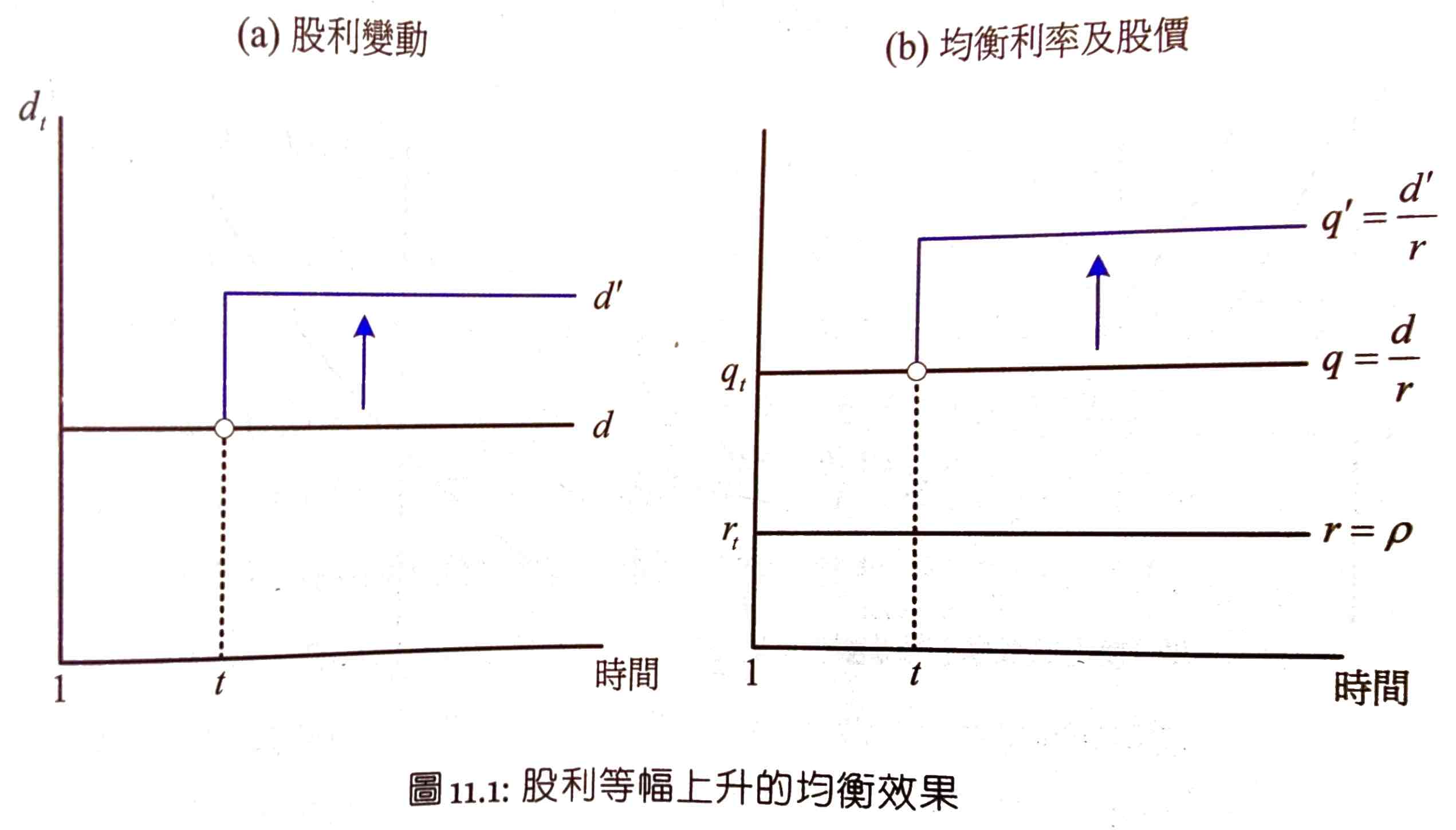
- saving demand no change
- bonds demand no change -> interest rate no change
- expected future stock price increases -> current stock demand increases -> stock price increases
- stock price \(q\) increases by the same ratio, \(q'=\dfrac{d'}{r}\)
- \(r=\dfrac{d'}{q'}\) no 套利空間
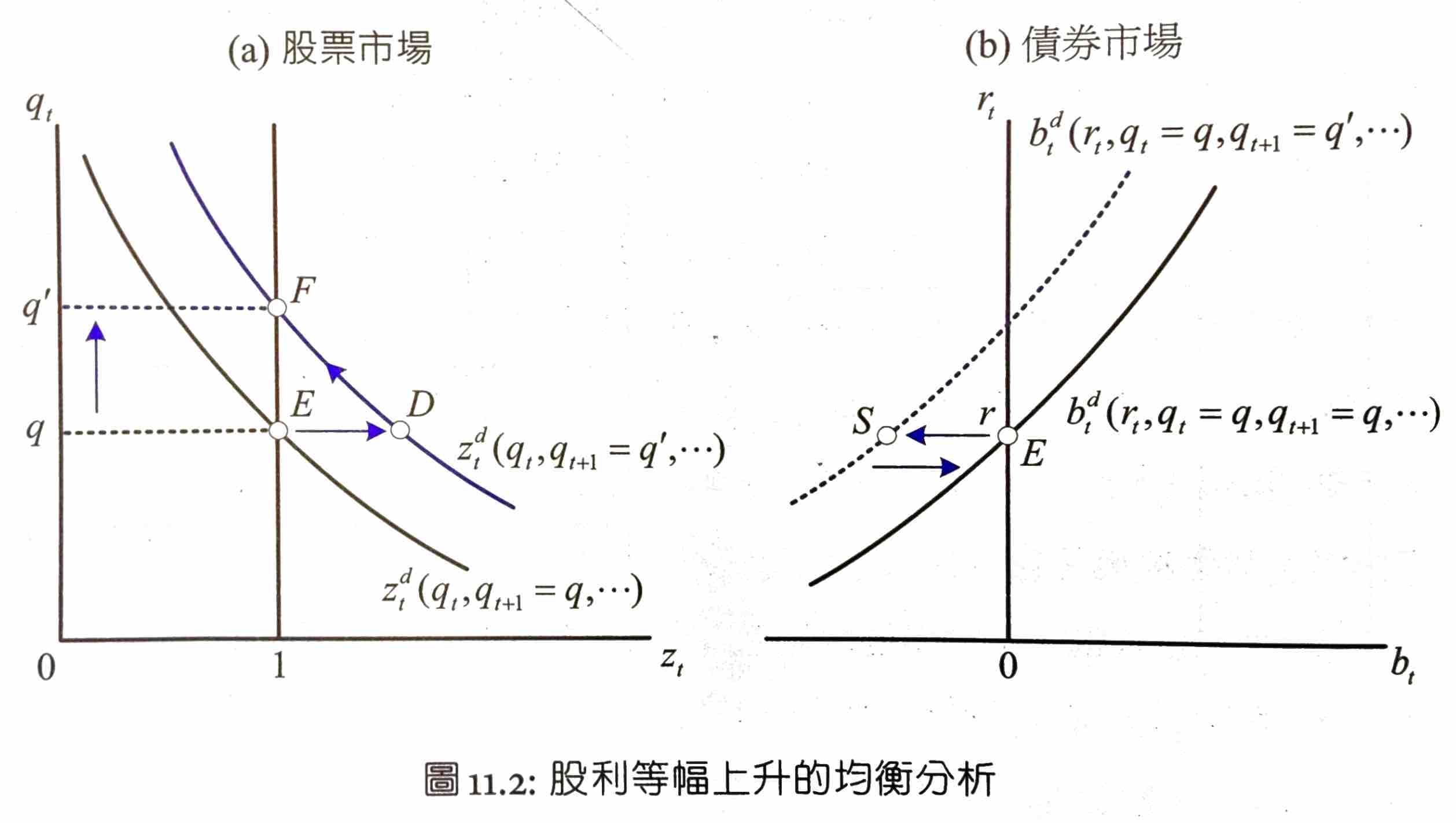
- bonds market
- E -> S: expected future stock price increase -> stock demand increases -> bonds demand decreases
- S-> E: stock demand > supply -> stock price increases -> bonds demand increases
- E -> S: expected future stock price increase -> stock demand increases -> bonds demand decreases
constant dividend growth
dividend growth rate = \(\mu\)
utility function (see #Problem 10.6)
assume \(\beta(1+\mu)^{1-\gamma}<1\) otherwise lifetime utility is infinite
-
0 when \(\gamma<1\)
- \(\gamma\) small -> 跨期 substitution effect 大
- income effect < 跨期 substitution effect
- = 0 when \(\gamma=1\)
- < 0 when \(\gamma>1\)
- \(\gamma\) big -> 跨期 substitution effect 小
- income effect > 跨期 substitution effect
income effect
expected future dividend increases -> saving demand decreases -> stock price decreases
跨期 substitution effect
expected future dividend increase -> stock demand increases -> stock price increases
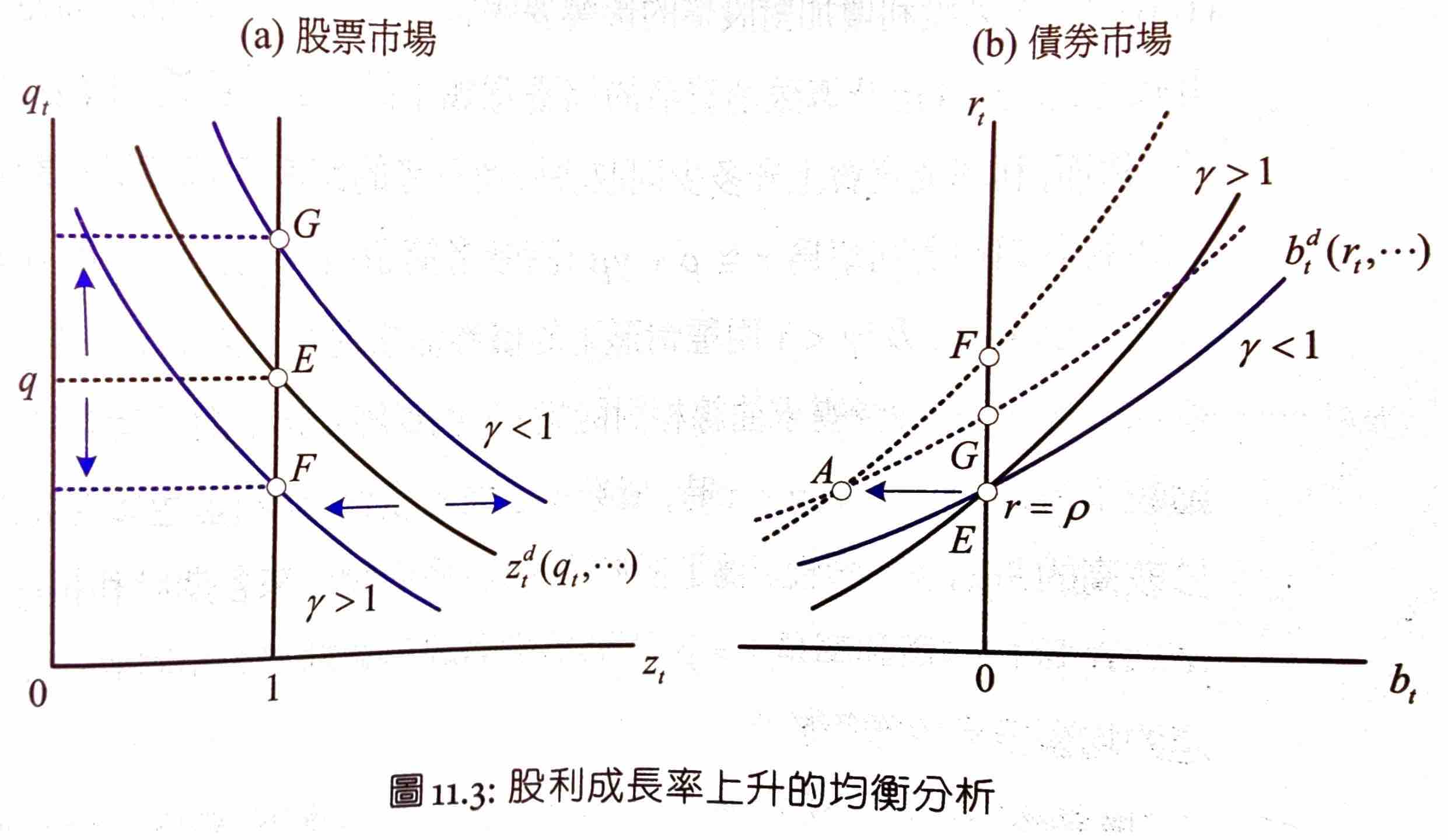
- bond market
- E -> A: income effect
- A -> F/G
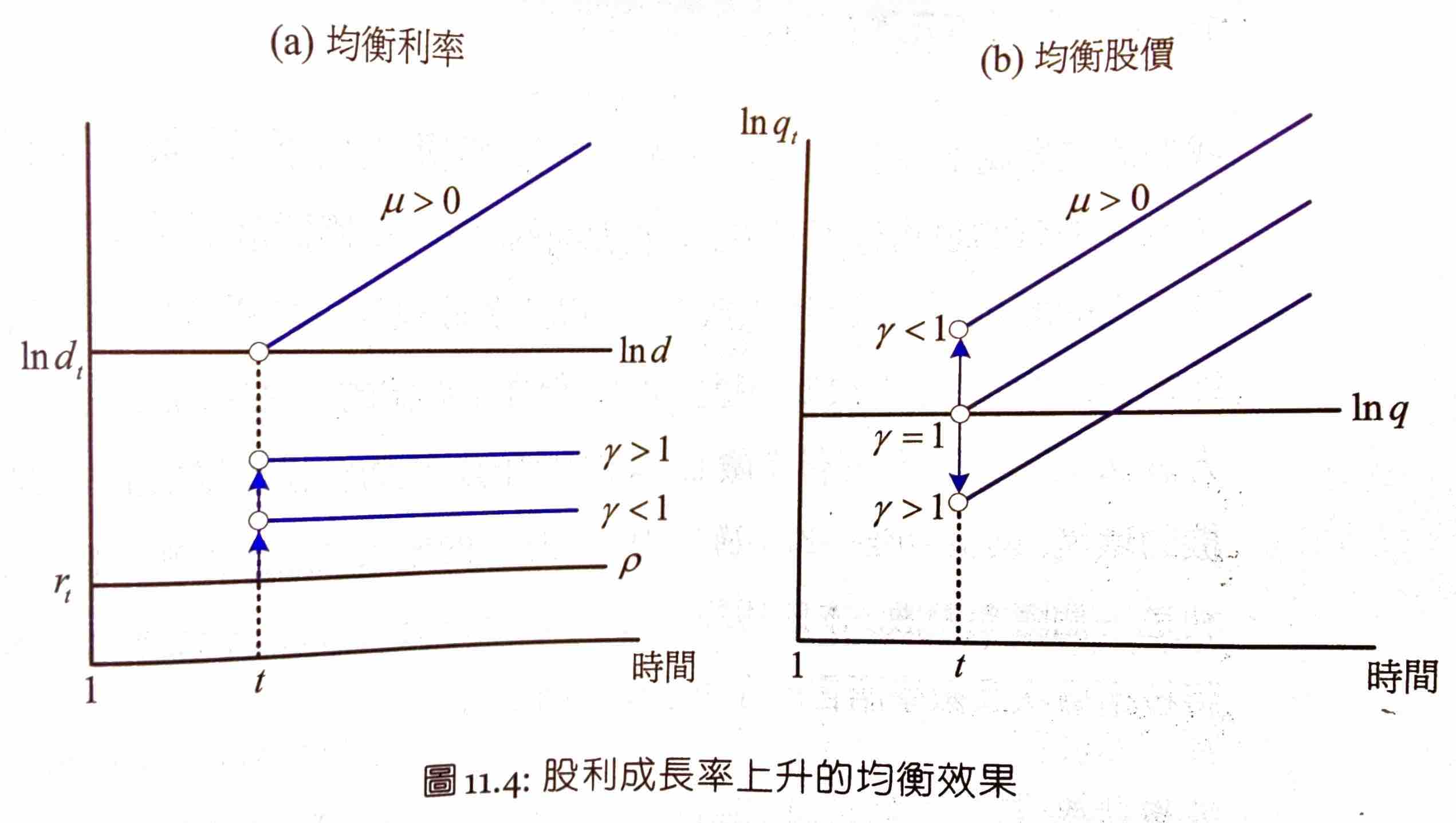
- \(q_t\) has the same growth rate as \(d_t\)
- \(\gamma > 1\) -> \(q_t\) smaller -> \(\dfrac{d_t}{q_t}\) & \(r\) higher
- \(\gamma=1\) -> \(q_t\) no change -> \(\dfrac{d_t}{q_t}\) & \(r\) higher
- \(\gamma<1\) -> \(q_t\) a bit bigger -> \(\dfrac{d_t}{q_t}\) & \(r\) higher
effects of government purchase
(from problem sets not main content)
Adding government purchase \(G_t\) to the model
government purchase temporarily increases
funding with fixed tax
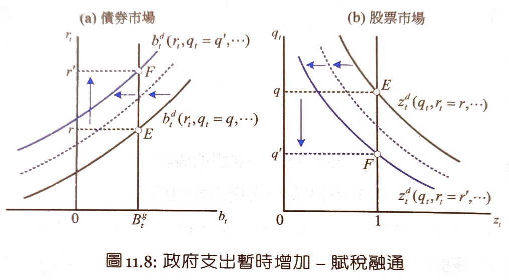
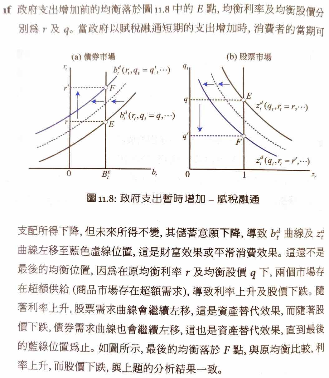
funding with bonds
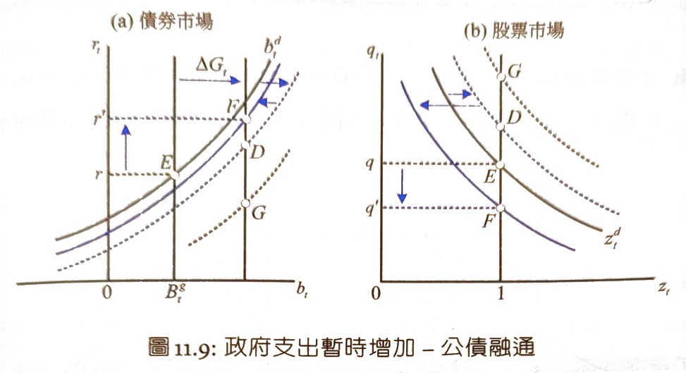
- income effect: E -> D
- future tax increases -> future income decreases -> current consumption decreases a bit -> current savings increases a bit -> bonds & stock demand increase a bit
- bonds interest rate increases greatly
- saving change < government purchase i.e. bonds supply change due to consumption smoothing
- 資產 substitution effect: D -> F
- bonds interest rate increases greatly -> stock demand decreases greatly
- overall stock price decreases moderately
- stock price decreases moderately -> bonds demand decreases moderately
- bonds interest rate increases greatly -> stock demand decreases greatly
- overall
- bonds interest rate rises
- stock price falls
government purchase permanently increases
Ch12 消費與勞動的跨期選擇
消費者的跨期選擇
consumers don't have endowment but work to earn
- \(l_t\) = time spend at leisure
- \(n_t\) = time spend at labore
- \(w_t\) = real wage (earnings per unit time of labor)
- \(d_t\) = dividends
- \(T_t\) = fixed tax, exogenous
- \(b_t\) = bonds at the end of period t
- \(r_t\) = real interest rate of bonds
- \(a_t\) = non-labor income = \(d_t-T_t\)
2-period budget constraint
savings
- \(b_0=0\)
- \(\lim_{t\rightarrow\infty}q_tb_t=0\)
- \(q_t=\prod_{i=1}^{t-1}(\dfrac{1}{1+r_i})\)
lifetime budget constraint
full wealth (if WLB = 0), treaing both consumption & leisure as commodities
optimization problem
first-order conditions
MRS of consumption & leisure = \(\dfrac{u_l}{u_c}=w_t\)
work 1 more unit time -> earn \(w_t\) more unit
consumption vs. future consumption
leisure vs. future consumption
work 1 more unit time -> earn \(w_t\) more unit -> buy bonds with them
consumption vs. future leisure
consume 1 less unit -> get \(1+r_t\) more future consumption, which translates to \(\dfrac{1+r_t}{w_{t+1}}\) of leisure
leisure vs. future leisure
work 1 more unit -> get \(w_t(1+r_t)\) more future consumption, which translates to \(\dfrac{w_t(1+r_t)}{w_t}\) of leisure
effects of exogenous variable changes
exogenous variables
- \(a_t\) non-labor income
- \(r_t\) real interest rate
- \(w_t\) real wage
effects of non-labor income change
\(a_t\) up -> lifetime wealth up -> consumption & leisure demands up, labor demand down for \(\forall t\)
Assume \(r_t=r\)
For temporary changes, income effect is weak
- \(\Delta y_t=\dfrac{r}{1+r}\Delta a_t\)
- \(\Delta c_t+w_t\Delta l_t\approx \Delta \bar{y_t}<\Delta a_t\)
- \(\Delta s_t=(\Delta a_t+w_t+r_{t-1}b_{t-1})-(\Delta c_t+w_tl_t)>0\)
For permanent changes, income effect is strong
- \(\Delta a_t=\Delta a \ \forall t\)
- \(\Delta y_t=\dfrac{r}{1+r}\Delta a\)
- \(\Delta c_t+w_t\Delta l_t\approx \Delta \bar{y_t}=\Delta a\)
- \(\Delta s_t=(\Delta a+w_t+r_{t-1}b_{t-1})-(\Delta c_t+w_tl_t)=0\)
effects of real interest rate change
\(\Delta r_t\) has no income effect but intertemporal substitution effect
real interest rate = cost of consumption
current real interest rate goes up ->
- current consumption down, future consumption up
- current leisure down, labor up
effects of real wage change
a change of wage has no income effect since it's zero sum among consumers and firms (wage up -> firm revenue/dividend down)
wage = cost of leisure
同期替代效果 contemporaneous substitution effect
current / forever wage up ->
- current / forever leisure down, labor up
- current / forever consumption up
intertemporal substitution effect
current wage up ->
- current leisure down, labor up
- future leisure up, labor down
future wage up ->
- current leisure up, labor down
- current consumption up
not existent when all periods are changed
effects on savings
\(w_t\) up ->
- \(n_t\) up, \(c_t\) up
- if intertemporal effect is very strong, then \(s_t\) up
\(w_{t+1}\) up -> \(n_t\) down, \(c_t\) up -> \(s_t\) down
if \(\Delta w_t = \Delta w \ \forall t\), the change on \(s\) can be ignored
equilibrium
government's budget constraint
firm's optimization problem
first-order
consumer's budget constraint
- \(d_t=y^s_t-w_tn^d_t\)
- \(T_t=G_t-b^g_t+(1+r_{t-1})b^g_{t-1}\)
- \(b_{t-1}=b^g_{t-1}\)
satisfies #Walras Law of Markets
MRS of consumption & leisure = wage = marginal productivity of labor
商品市場結清條件
*National Savings
private saving
government saving
in a closed economy \(b^g_t=b_t\)
national saving
\(S=I+CA\) but in this economy there's no investment nor international trades so \(S=I=CA=0\)
So the economy cannot save anything, everything have to be consumed immediately.
Compared to 靜態模型, there's a loan market. Compared to the endowment model, there's a labor market. The additional variables, however, are all endogeneous.
Simplification
labor market 結清條件
consumption market 結清條件
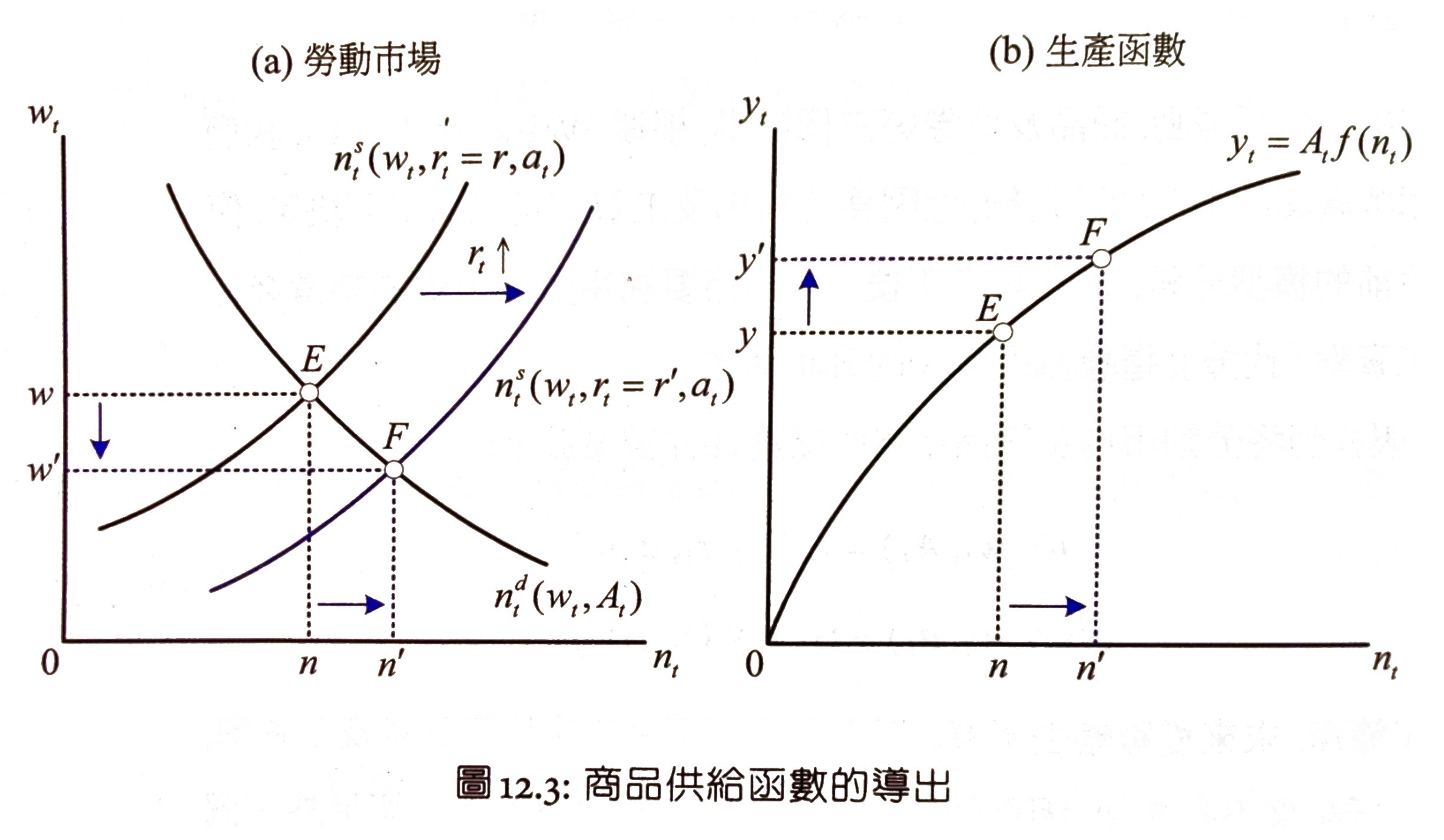
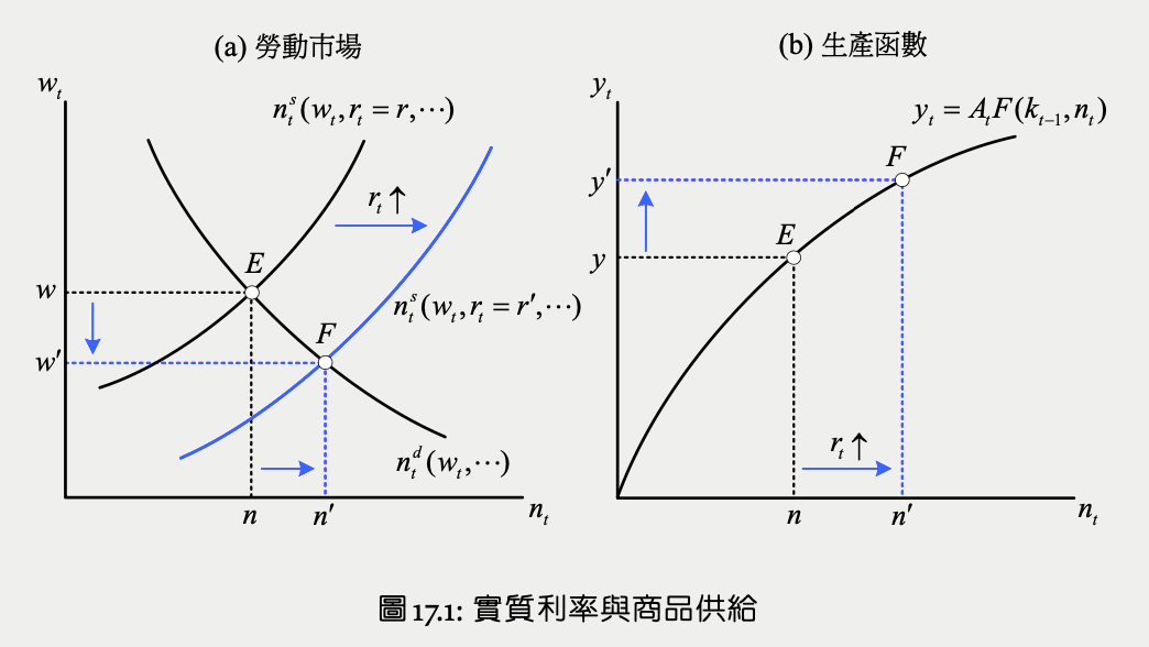
\(r\) up -> labor supply \(n^s_t\) right shift -> \(w\) down \(n\) up -> \(y\) up
so \(y^s_t\) up when
- \(r_t\) up
- \(A_t\) up
- \(a_t\) down
as long as consumption & labor market are in equilibrium, bond market will also be
short-term equilibrium
The model in this chapter is like the super-short term scenario in real life, where firms cannot change its capital i.e. invest
temporary supply shock
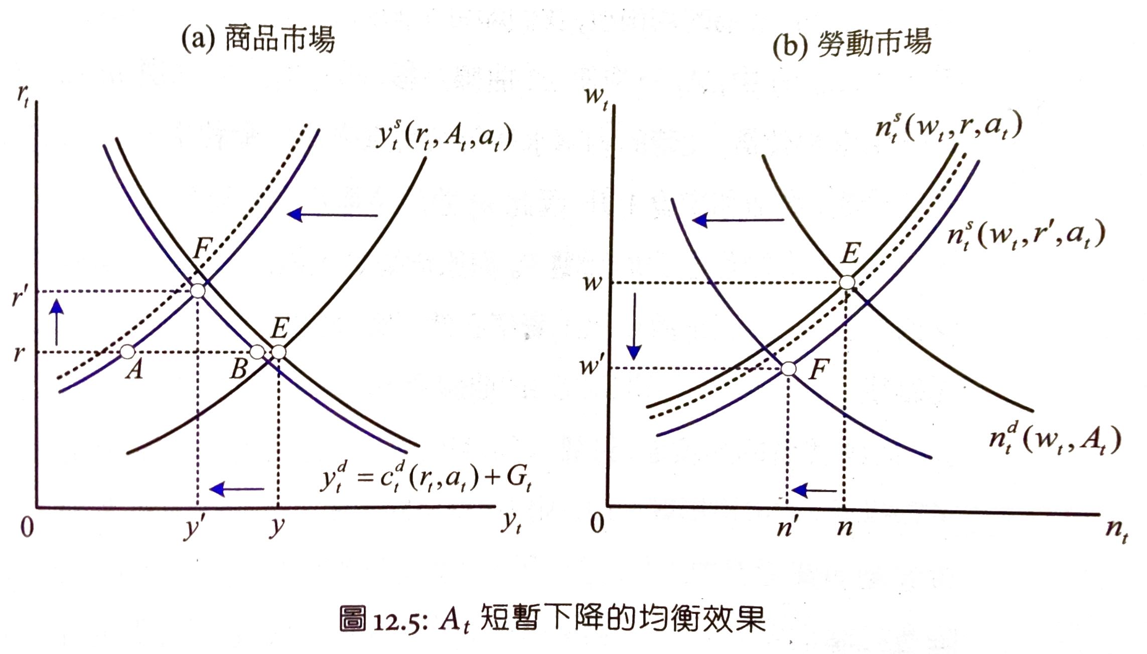
\(A_t\) down ->
- consumption market
- direct effect: \(y^s_t\) left shifts
- income effect: \(a_t\) down -> consumption down, leisure down, labor up -> \(y^d_t\) left shifts a bit, \(y^s_t\) right shifts a bit (consumption smoothing)
- demand > supply in consumption market due to consumption smoothing
- supply > demand in bond market -> interest rate up
- intertemporal substitution effect: \(r\) up -> consumption demand down B to F, commodity supply up A to F
- labor market
- \(n^d_t\) left shifts
- income effect: \(n^s_t\) right shifts
- equilibrium
- \(w\) down
- \(n\) depends
- if consumers are very sensitive to wage, then labor down
No investment so the shock is consumed entirely in this period. Future periods are not affected.
expected future shock
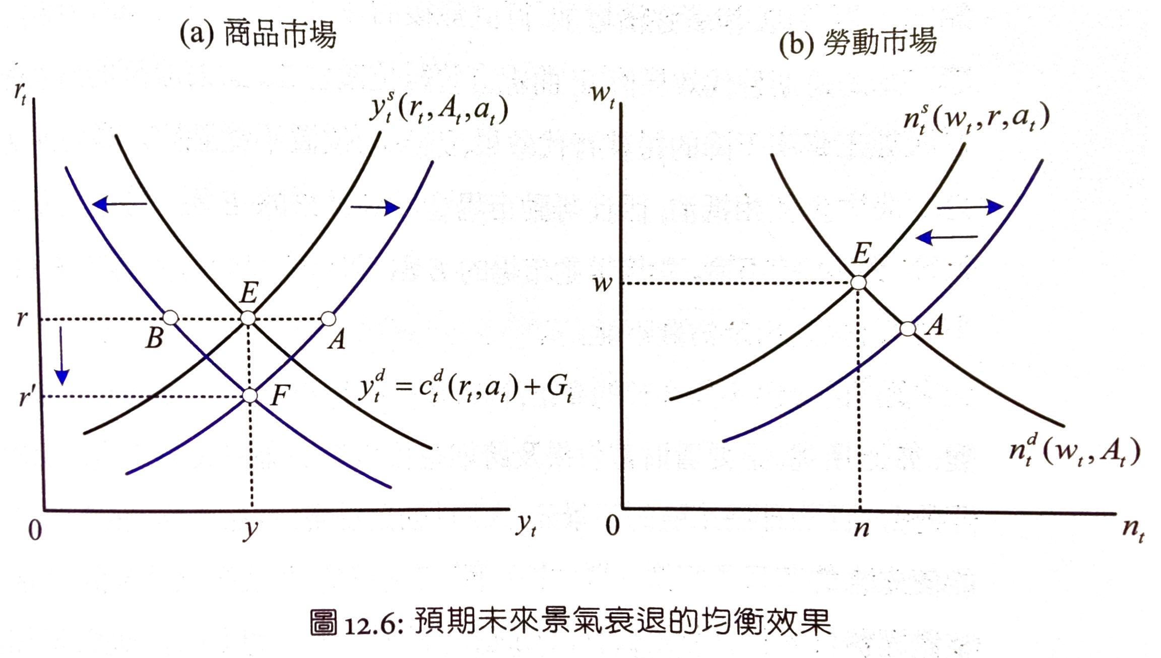
\(A_{t+1}\) down ->
- labor market
- \(A_t\) unchanged so \(n^d_t\) unchanged
- income effect: consumption down, leisure down, labor up -> \(n^s_t\) right shifts
- intertemporal substitution effect: \(w_{t+1}\) down -> \(n^s_t\) right shifts
- consumption market
- income effect & intertemporal substitution effect: \(y^d_t\) left shifts
- supply > demand
demand > supply in bond market -> interest rate down
intertemporal substitution effect:
- commodity market: \(r\) down -> consumption demand up B to F, commodity supply down A to F
- labor market: \(r\) down -> \(n^s_t\) left shifts, may or may not exceed E
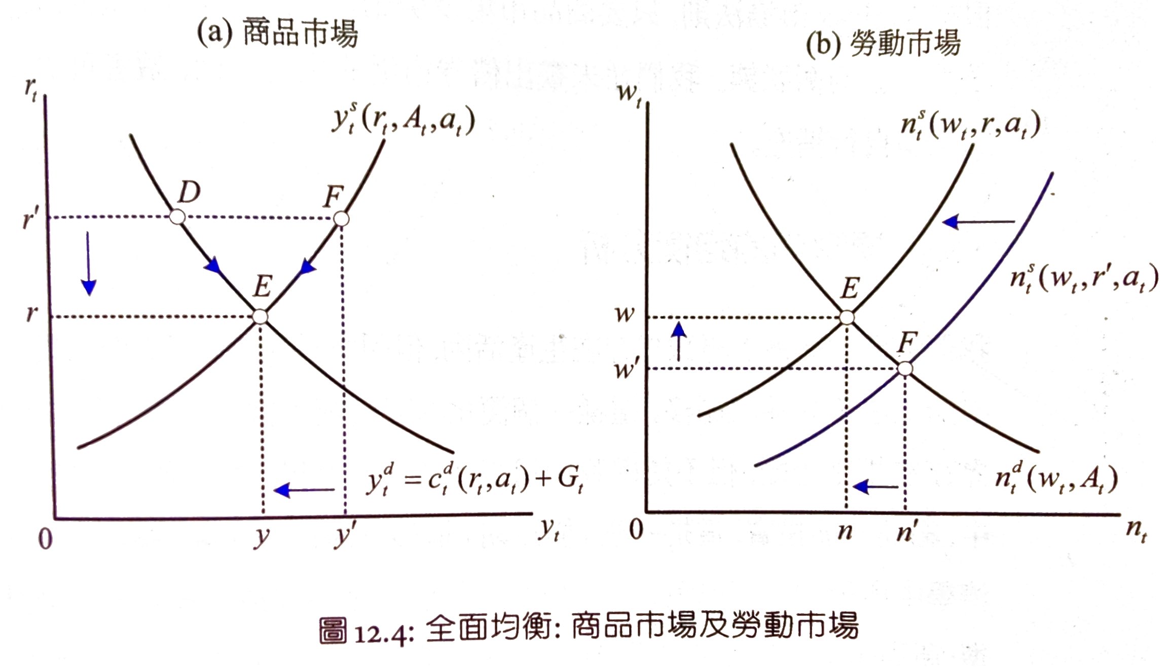
temporary demand shock
government increases expenditure during recession
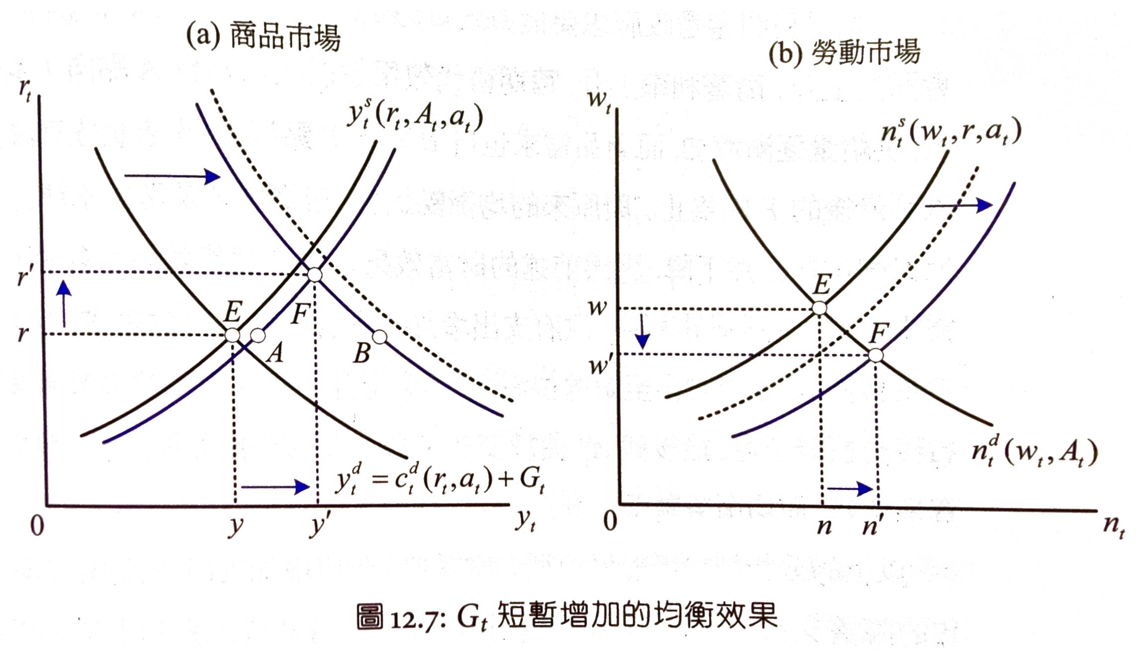
\(G_t\) up
- commodity market
- direct effect: \(y^d_t\) left shifts
- income effect: tax up -> consumption down, leisure down, labor up -> \(y^d_t\) left shifts a bit, \(y^s_t\) right shifts a bit (consumption smoothing)
- demand > supply
- labor market
- income effect: \(n^d_t\) right shifts
supply > demand in bond market -> interest rate up
intertemporal substitution effect:
- commodity market
- \(r\) up -> \(y^s_t\) right shifts A to F, \(y^d_t\) left shifts B to F
- labor market
- \(r\) up -> \(n^d_t\) right shifts
equilibrium
- consumer lifetime wealth down
- wage down
- interest rate up
- private consumption down - 排擠效果
- consumer lifetime utility down
Ch13 廠商的投資決策 Ramsey Model
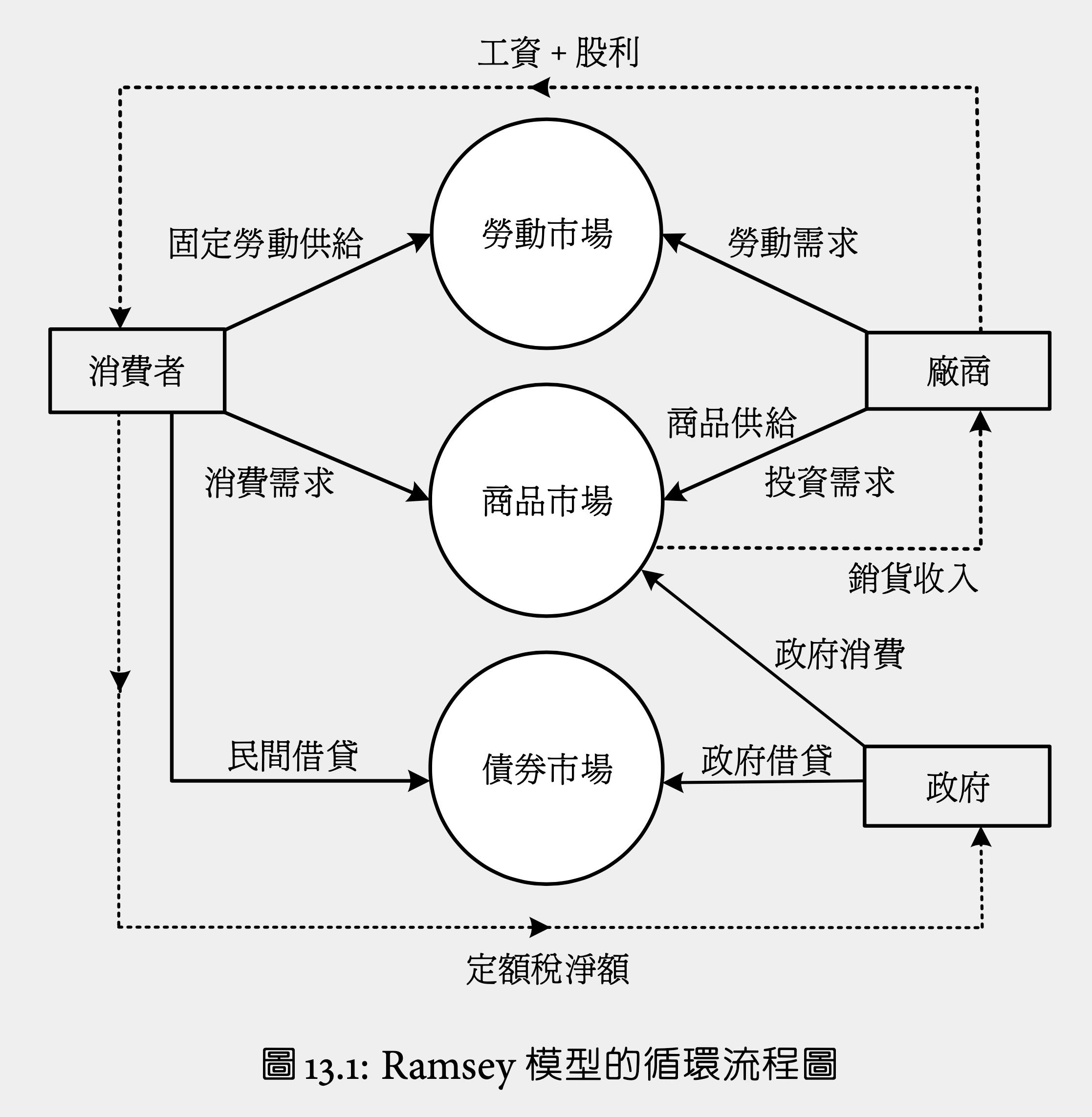
- aliases
- Ramsey-Cass-Koopmans Model
- optimal growth model
- similar to #Ch12 消費與勞動的跨期選擇 except
- Ch12: consumers can decide labor supply, firms can't invest
- Ch13: consumers can't decide labor supply, firms can invest i.e. accumulate capitals
- goods can be consumed or accumulated i.e. served as investment
- exogenous variables
- total factor productivity \(A_t\)
- government policy \(G_t\) & \(T_t\)
- endogeneous variables
- wage \(w_t\)
- interest rate \(r_t\)
- consumption \(c_t\)
- investment \(i_t\)
- production \(y_t\)
- capital \(k_t\)
- labor \(n_t\)
- equilibrium number, not supply
- bonds \(b_t\)
consumer
Budget constraint
where \(a_t=d_t+w_t-T_t\) = exogenous income
lifetime
utility optimization
first order
government
government budge constraint
lifetime
firm
- \(k_{t-1}\) = capital @ beginning of the period
- \(n_t\) = labor
- \(A_t\) = total factor productivity 要素生產力 or 供給面衝擊
- exogenous
- \(F\) satisfied 古典假設
- constant return to scale
- individual firm's behaviour can represent the whole society's production
law of motion of capital
- \(i_t\) = firm's investment
- \(\delta\) = depreciation rate of capital
(gross) investment = net investment + depreciation
value of firm
As dividends will fall into shareholders' pockets eventually, the lifetime value of total dividends is what consumers care about
cash flow = revenue - labor cost - investment
lifetime dividends optimization
first-order condition
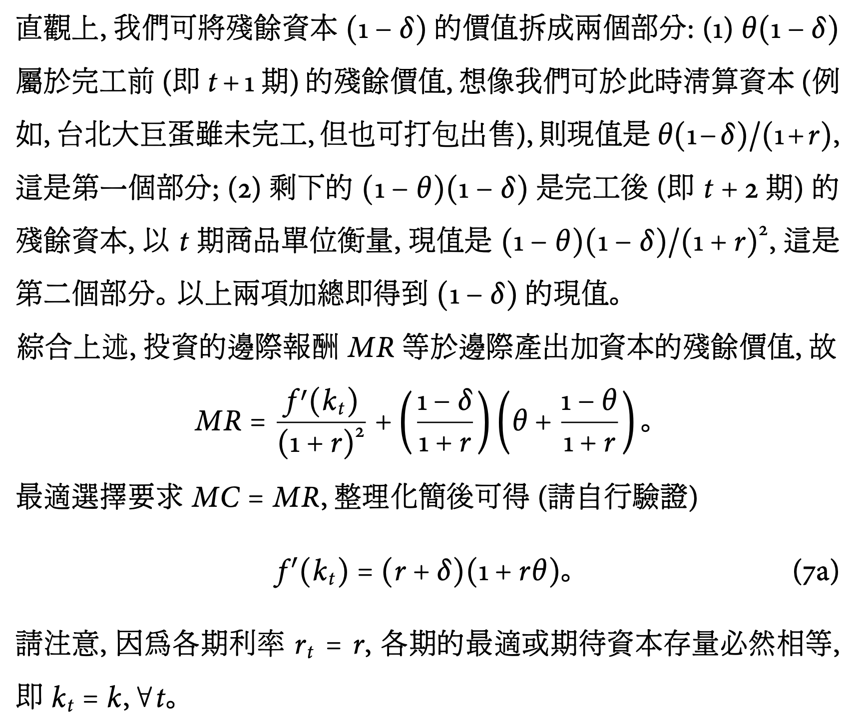
marginal productivity of labor = wage
effect of one unit of additional investment
- change of current cash flow = -1
- change of future cash flow = future marginal productivity of capital MPK + residual or liquidation value of capital
fuure MPK = opportunity cost of investment
bond gain = capital investment net gain
cost of external financing = cost of internal financing
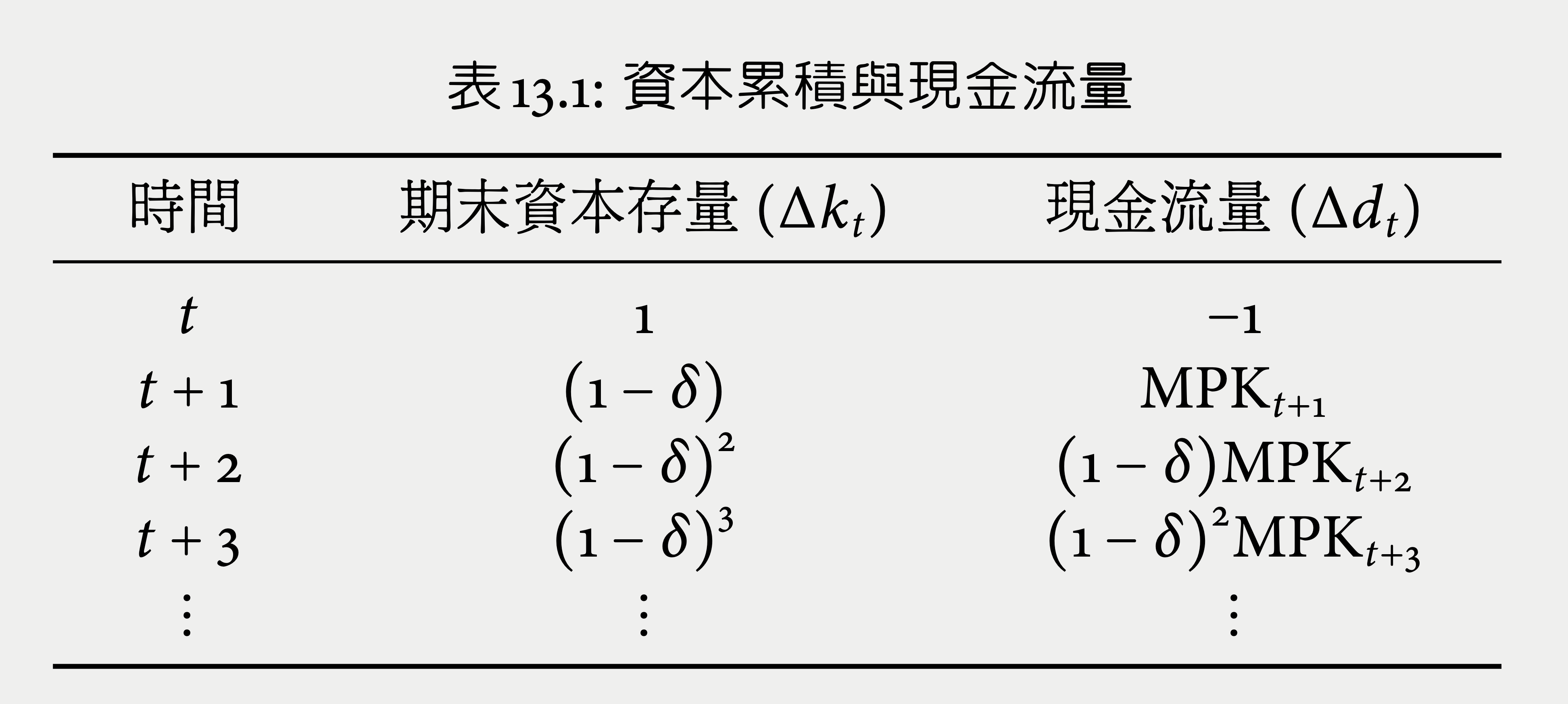
one unit of investment = change of lifetime dividents
meaning either the firm continues to operate forever or shuts down at next period, it's the same
investment demand
real interest rate up
E->B: \(r\) up -> cost of investment up -> desired capital stock \(k^*_t\) down -> investment down
investment elasticity against real interest rate irl is very high
- capital-investment ratio is very low (about 15:1 irl)
- -> a tiny change in capital is a huge change in investment
depreciation ratio up
\(\delta\) up -> desired capital stock \(k^*_t\) net investment down -> gross investment = net investment + depreciation not definitively up or down
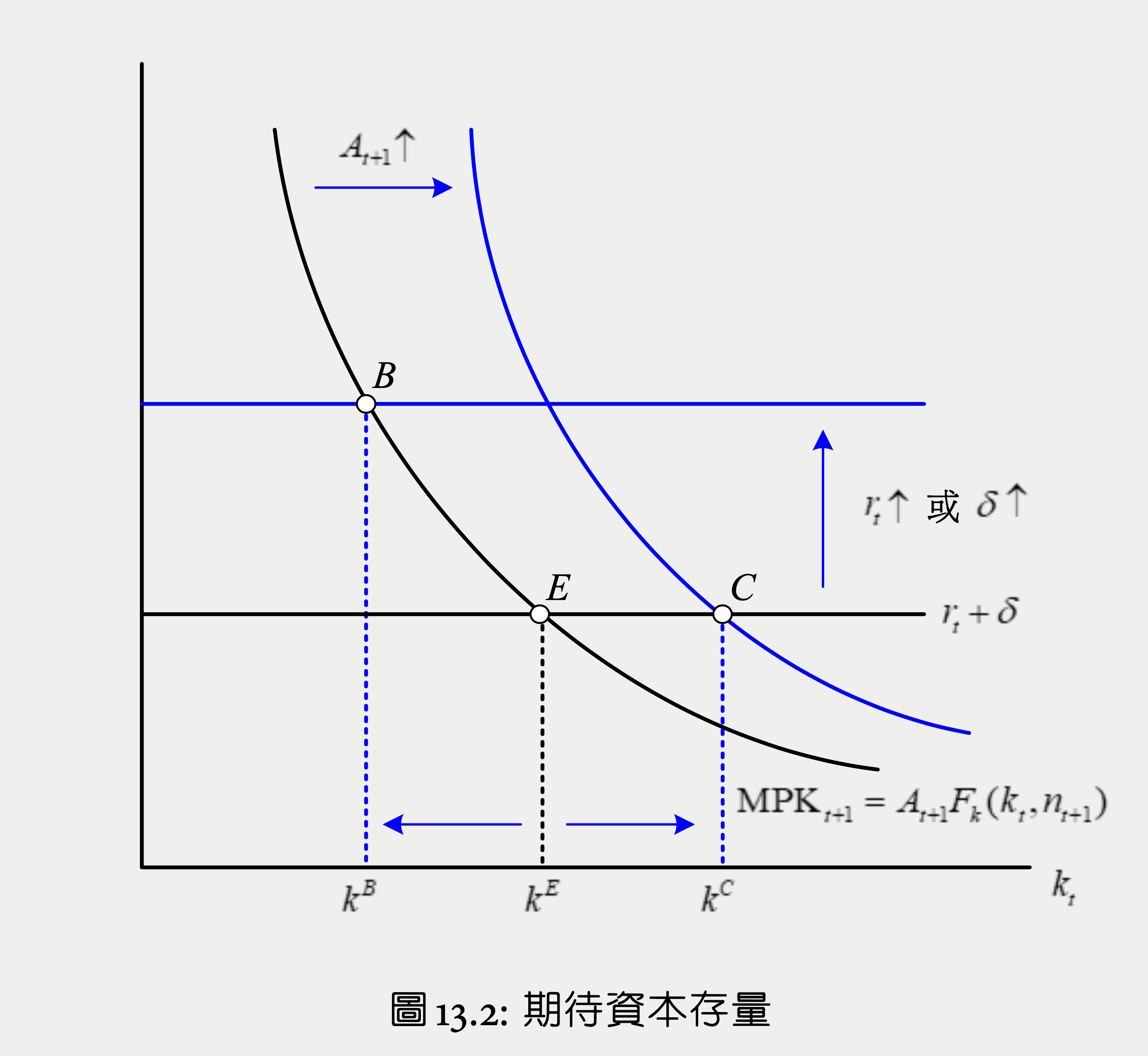
expected 要素生產力 up
\(\mathrm{MPK}_t=A_tF_k(k_{t-1},n_t)\) does not affect today's investment demand as it's not related to 期末 capital \(k_t\), but \(\mathrm{MPK}_{t+1}=A_{t+1}F_k(k_{t},n_{t+1})\) does
E -> C: \(A_{t+1}\) up -> \(\mathrm{MPK}_{t+1}\) up -> desired capital stock up -> investment up
期初 capital down
\(k_{t-1}\) down ->
- \(i_t=k^*_t-(1-\delta)k_{t-1}\) up
- intuition: buy more to fill the hole
- \(\mathrm{MPK}_t=A_tF_k(k_{t-1},n_t)\) up
- \(\mathrm{MPK}_{t+1}=A_{t+1}F_k(k_{t},n_{t+1})\) no change -> \(k^*_t\) no change
overall investment demand curve
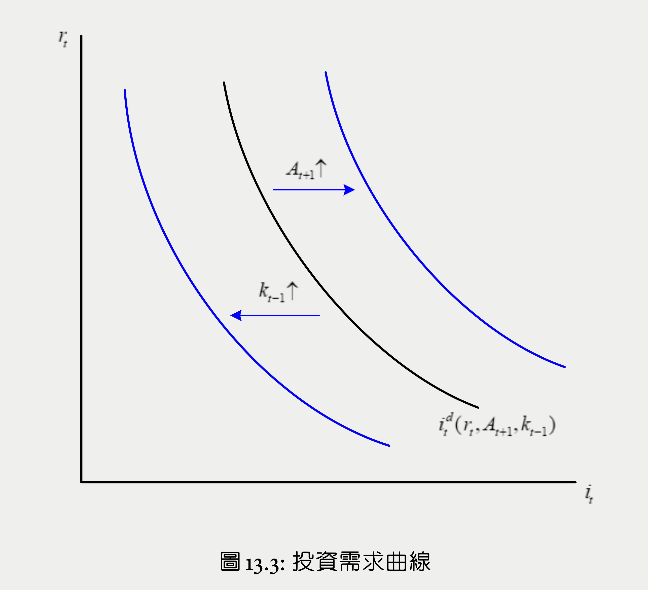
investment demand \(i^d_t\) up when
- \(r_t\) down
- \(A_{t+1}\) up
- \(k_{t-1}\) down
- \(\delta\) depends
investment tax credit
simplify the production function by ignoring labor & factor productivity
assume tax credit i.e. deduction = \(\phi_t\in(0,1)\)
actual investment expenditure = \((1-\phi_t)i_t\)
cash flow = production - investment expenditure
so tax deduction increases cash flow
optimization problem
1 unit of capital at period \(t\) can be sold \(1-\phi_t\) (residual value)
marginal cost of investment = marginal profit
MPK = opportunity cost of investment - residual value
when \(\phi_t=\phi \ \forall t\)
\(\phi\) permanently up -> capital & investment demand up
effect of tax deduction rate change
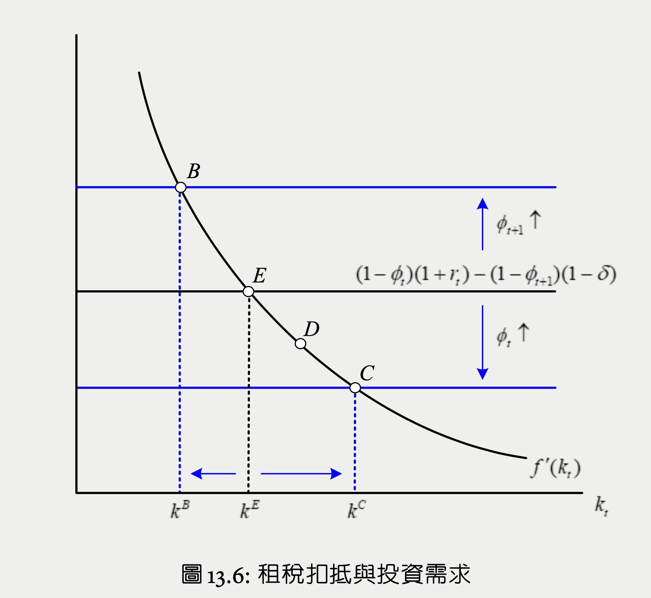
- E -> \(\phi_t\) up -> cost of investment shifts down -> C
- E -> \(\phi_{t+1}\) up -> cost of investment shifts up -> B
- residual value of today's investment \((1-\phi_{t+1})(1-\delta)\) down
- E -> \(\phi\) permanently up -> D
- \(\Delta\phi(1+r_t)>\Delta\phi(\delta+r_t)\)
Example
Assuming \(r_t=r\), \(f(k)=k^\alpha\), \(\alpha\in(0,1)\)
when \(\phi_t=\phi\)
elasticity for permanent investment deduction
if originally there's no investment deduction i.e. \(\phi=0\)
when \(\phi_t\) is differencing for each \(t\)
if originally there's no investment deduction i.e. \(\phi_t=\phi_{t+1}=0\)
general equilibrium 全面均衡
solving endogeneous variables
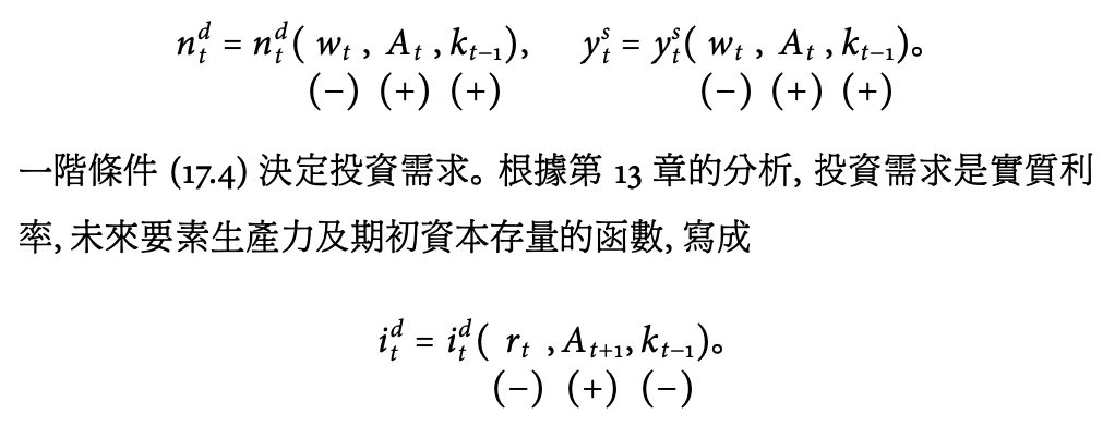
deriving \(w_t,y_t,n_t,b_t\)
- max consumer utility
- \(u'(c_t)=\beta u'(c_{t+1})(1+r_t)\)
- \(c_t+b_t=(d_t+w_t-T_t)+(1+r_{t-1})b_{t-1}\)
- max firm value
- \(\mathrm{MPL}_t=A_tF_n(k_{t-1},n_t)=w_t\)
- \(=A_tF_n(k_{t-1},1)\), which is dependent on exogenous variables only
- \(k_{t-1}\) is exogenous since it's from the past, you can do nothing to change it
- \(=A_tF_n(k_{t-1},1)\), which is dependent on exogenous variables only
- \(\mathrm{MPK}_{t+1}=A_{t+1}F_k(k_{t},n_{t+1})=r_t+\delta\)
- \(\mathrm{MPL}_t=A_tF_n(k_{t-1},n_t)=w_t\)
- government budget constraint
- \(G_t+(1+r_{t-1})b^g_{t-1}=T_t+b^g_t\)
- market demand = supply
- \(n^d_t=n^s_t=1\)
- \(b^d_t=b^s_t=1\)
- \(c^d_t+i^d_t+G_t=y^s_t\)
- \(y_t=A_tF(k_{t-1},n_t)=A_tF(k_{t-1},1)=A_tf(k_{t-1})\)
deriving \(r_t,c_t,i_t,k_t\)
- \(u'(c_t)=\beta u'(c_{t+1})[A_{t+1}f'(k_t)+(1-\delta)]\)
- \(c_t+[k_t-(1-\delta)k_{t-1}]+G_t=A_tf(k_{t-1})\)
national saving
private budge constraint
private saving
public saving
\(b_t=b^g_t \ \forall t\) in a closed economy
national saving
In a closed economy, investment solely comes from national saving
Crusoe
Ramsey-Crusoe mapoing
- spend a fixed time collecting fruits each day \(y_t=A_tf(k_{t-1})\)
- \(A_t\) is the mother nature factor
- \(k_{t-1}\) is the seeds you planted yesterday, which will grow to fruits in a day
- a fruit can either be eaten xor be planted as a seed
- grown fruits still need to be collected to be utilized
- \(\delta\) of seeds are eaten
- \(G_t\) fruits are stolen
- \(k_t=i_t+(1-\delta)k_{t-1}\)
- \(y_t=c_t+i_t+G_t\)
utility optimization problem
\(\(\max_{\{c_t,k_t\}^\infty_{t=1}}=\sum^\infty_{t=1}\beta^{t-1}u(c_t)\)\) first-order
limitations of Ramsey Model
Production this period is decided by the previous period, so it won't be affected by future perturbations, which is unrealistic.
Problems
P3
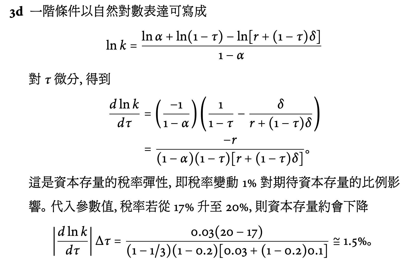
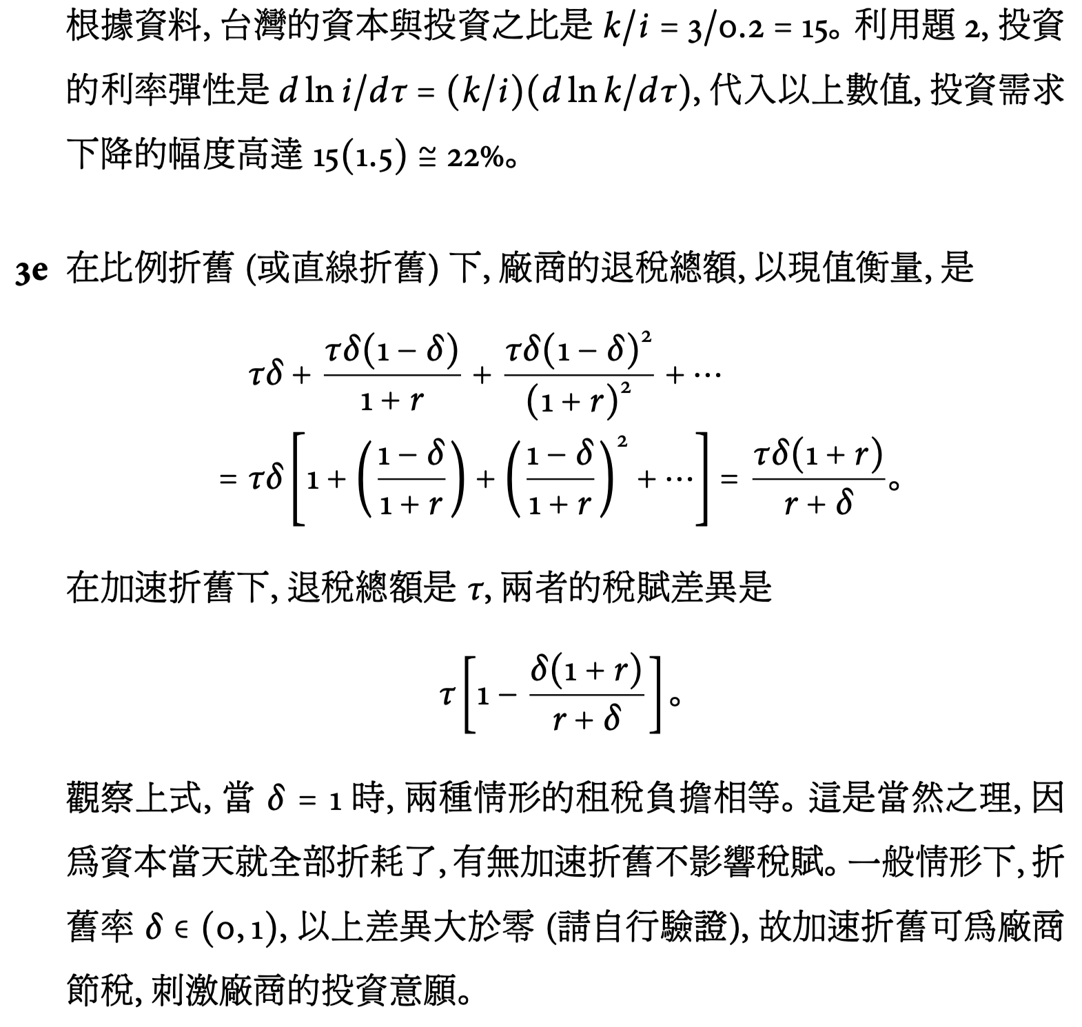
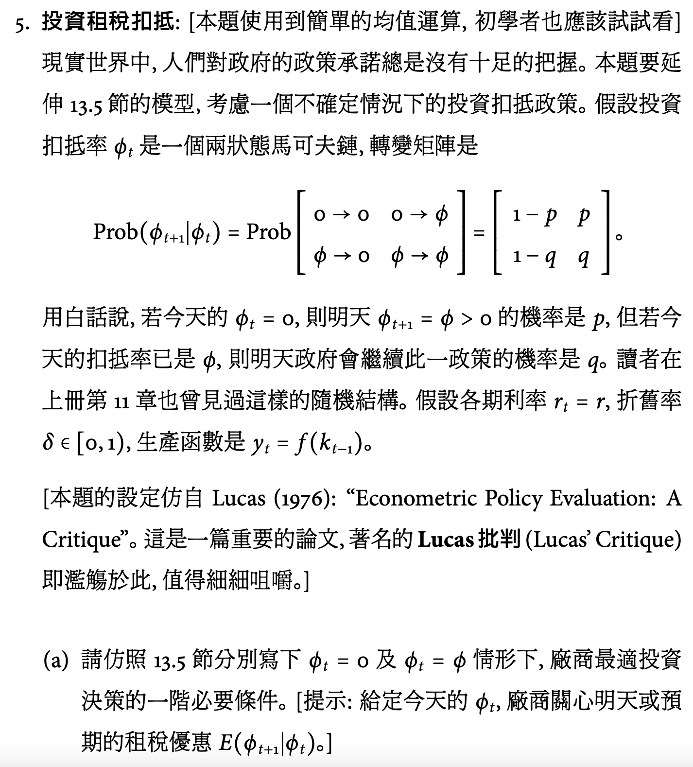
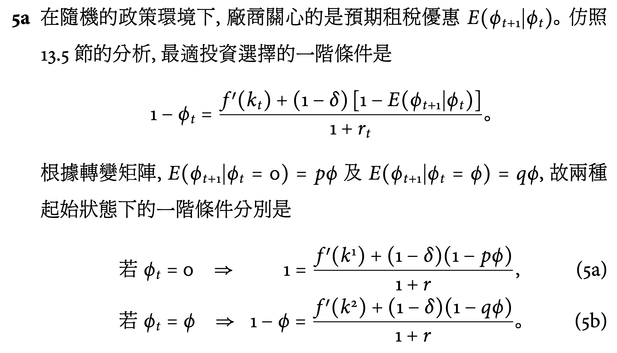
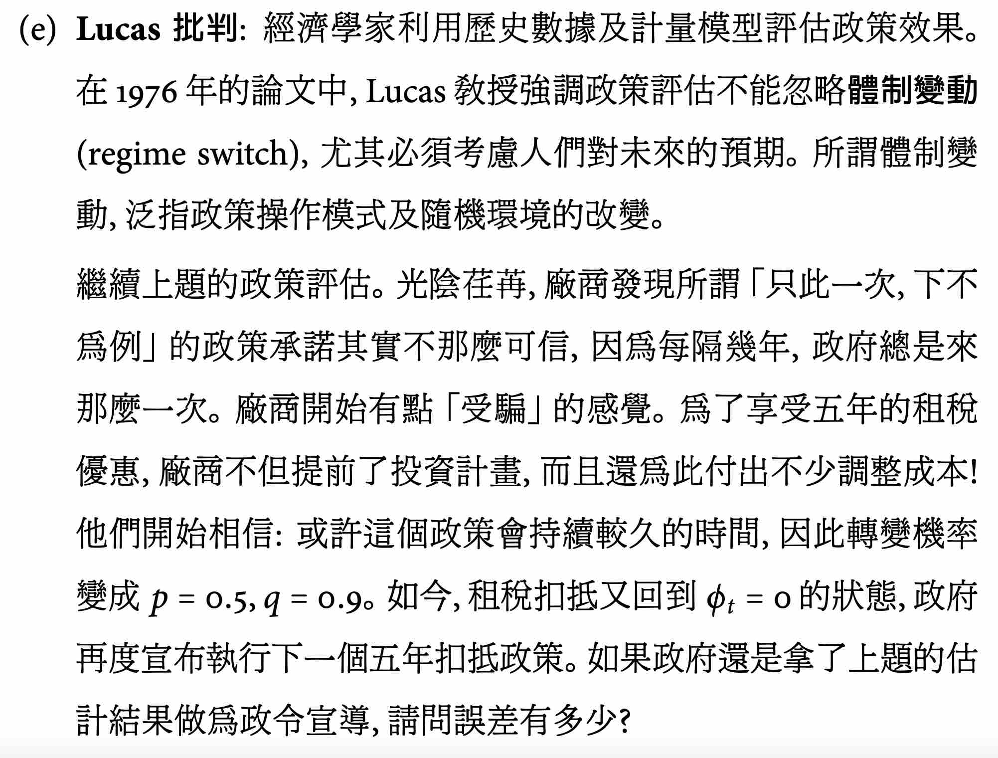
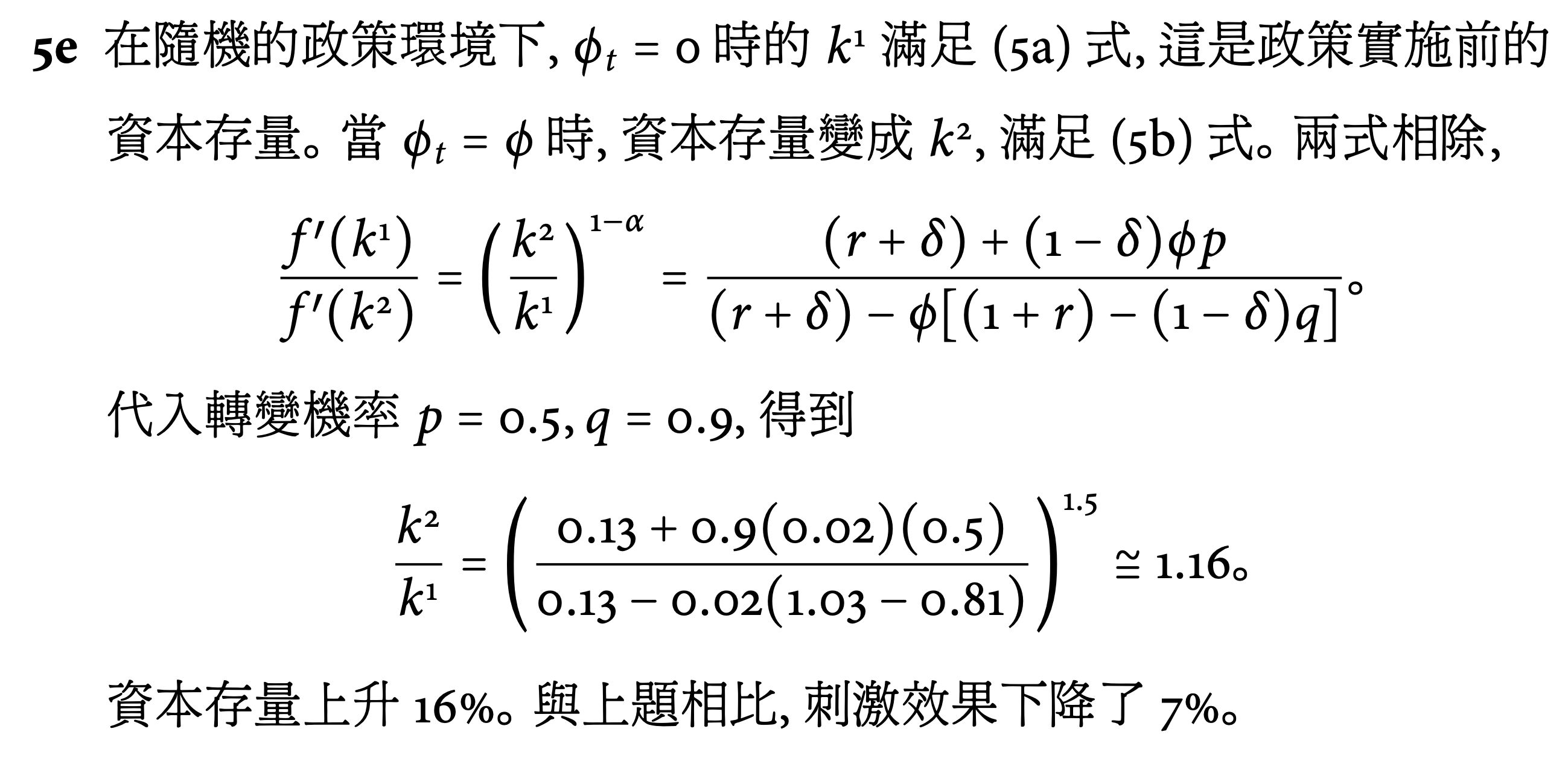
P5 Lucas' Critique
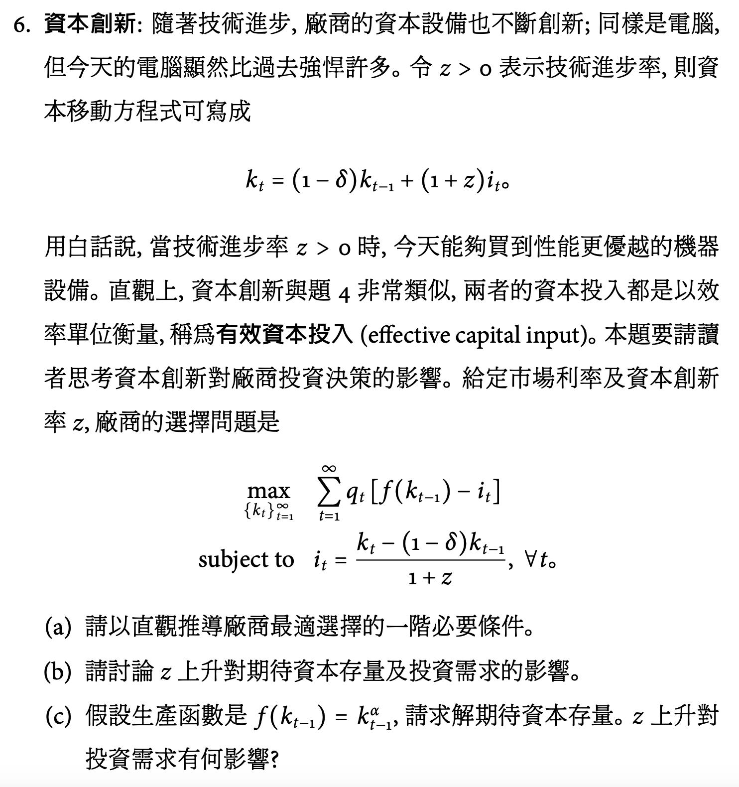
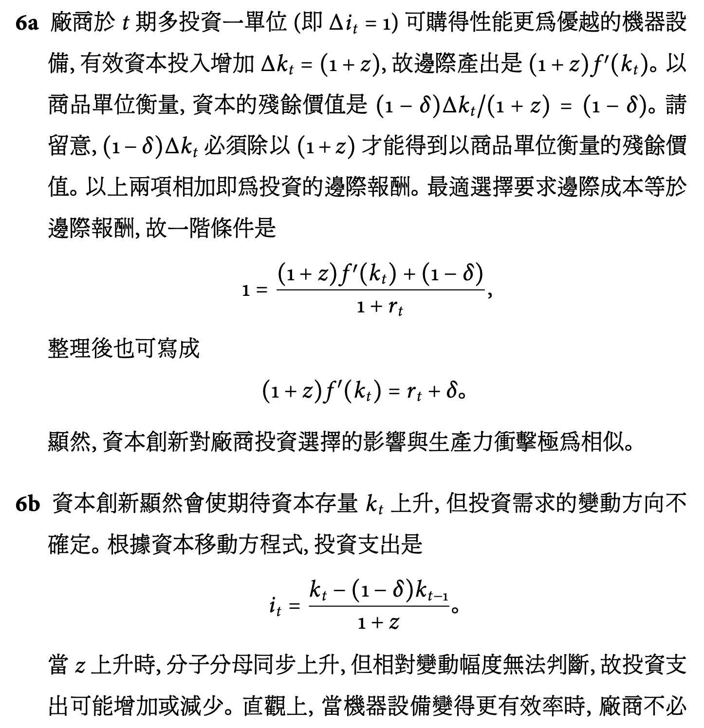
P6
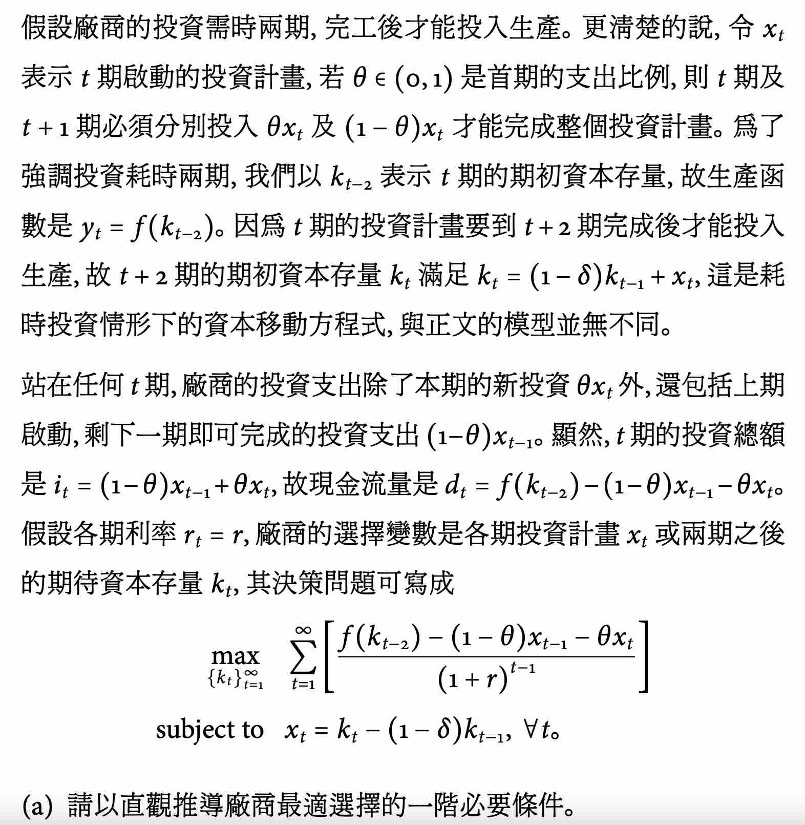
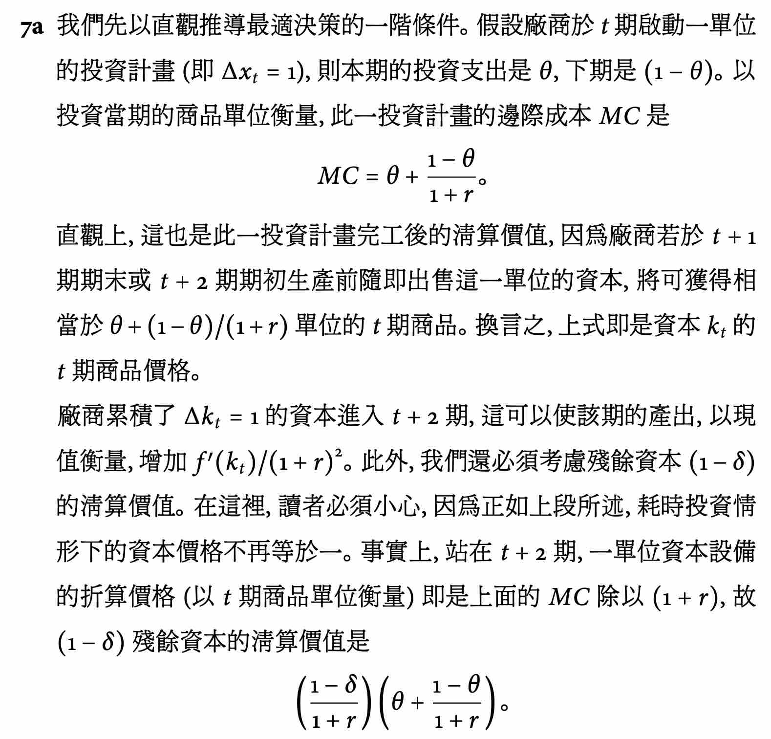
P7 time-to-build
Ch17 Real Business Cycle RBC Model
Real Business Cycle (RBC) Model = Ramsey Model + endogenous labor supply
consumer
#Ch13 廠商的投資決策 Ramsey Model#consumer but with wage & labor as endogenous variables
Budget constraint
where
- \(a_t=d_t-T_t\) = exogenous non-labor income
- \(n_t+l_t=1\)
lifetime
完全財富
utility optimization
first order
See also #Ch12 消費與勞動的跨期選擇#消費者的跨期選擇
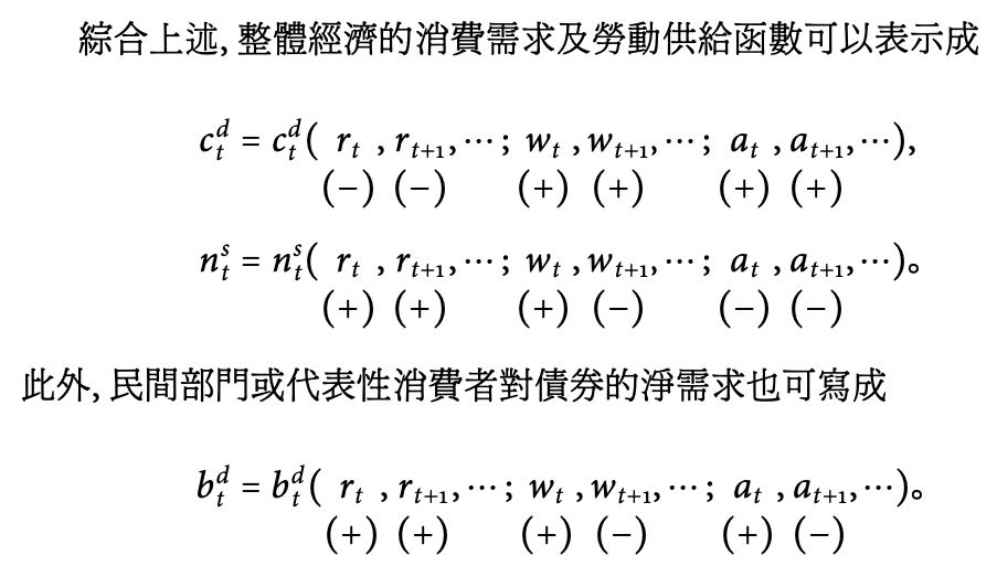
effect of exogenous variable changes
- non labor income up
- income effect: consumption demand up, leisure demand up, labor supply down
- \(a_t\) up -> savings up -> \(b^d_t\) up
- \(a_{t+1}\) up -> savings down -> \(b^d_t\) down
- \(a\) permanently up -> savings & bonds demand no change
- real interest rate up
- no income effect but intertemporal substitution effect
- \(r\) up -> consumption & leisure's opportunity cost up -> \(c^d_t\) & \(l^d_t\) down, \(n^d_t\) up
- real wage up
- no income effect
- zero sum between consumer & firm
- contemporaneous substitution effect: \(w_t\) up -> \(n_t\) & \(c_t\) up
- intertemporal substitution effect
- \(w_t\) up -> \(n_t\) up
- \(w_{t+1}\) up -> \(n_t\) down, \(c_t\) up
- \(w\) permanently up -> no change
- no income effect
firm
same as #Ch13 廠商的投資決策 Ramsey Model#firm
government
same as #Ch13 廠商的投資決策 Ramsey Model#government
government budge constraint
lifetime
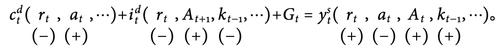
general equilibrium
#Ch13 廠商的投資決策 Ramsey Model#general equilibrium 全面均衡 but with wage & labor as endogenous variables
Deciding \(w_t,r_t,c_t,n_t,k_t\)
- market clearing conditions
- \(n^d_t=n^s_t\)
- \(b^d_t=b^s_t\)
- \(c^d_t+i^d_t+G_t=y^s_t\)
simplify
- contemporaneous SE: \(\dfrac{u_l(c_t,l_t)}{u_c(c_t,l_t)}=A_tF_n(k_{t-1},n_t)\)
- \(\mathrm{MPL}_t=A_tF_n(k_{t-1},n_t)=w_t\)
- intertemporal SE: \(u_c(c_t,l_t)=\beta u_c(c_{t+1},l_{t+1})[A_{t+1}F_k(k_{t},n_{t+1})+(1-\delta)]\)
- \(u_c(c_t,l_t)=\beta u_c(c_{t+1},l_{t+1})(1+r_t)\)
- \(\mathrm{MPK}_{t+1}=A_{t+1}F_k(k_t,n_{t+1})=r_t+\delta\)
- budget: \(c_t+[k_t-(1-\delta)k_{t-1}]+G_t=A_tf(k_{t-1}, n_t)\)
- \(i_t=k_t-(1-\delta)k_{t-1}\)
Crusoe
#Ch13 廠商的投資決策 Ramsey Model#Crusoe but he can decide his labor time
utility optimization problem
first-order
consumer & labor market
since it's wage vs. labor in the labor market, interest rate change causes the curve to move not just the point as in consumer market
steady-state
every endogenous variables in each period stays the same
example
Given
- \(u(c,l)=\ln c+\ln l\)
- \(y=Ak^\alpha n^{1-\alpha}, \alpha\in(0,1)\)
- \(G=gy, g\in(0,1)\)
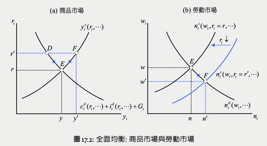
capital-production ratio \(\phi=\dfrac{\alpha}{\rho+\delta}\) is a constant
substitute into \(c^*+\delta k^*+G=y^*\)
MRS = MPL
solving \(n^*,y^*,k^*,c^*,w^*\)
effect of total factor productivity change
when total factor productivity \(A\) is up
- substitution effect: \(A\) up -> MPL up -> \(c\) up & \(l\) down, \(n\) up
- income effect: \(A\) up -> \(c\) & \(l\) up, \(n\) down
- no intertemporal substitution effect as \(r=\rho\)
effects
- the change of \(n\) depends
- it is generally small as SE & IE work against each other
- it is cancelled out under logrithmic utility function & Cobb-Douglas production function in #Ch17 實質循環模型 Real Business Cycle Model#example
- \(c\) up
effect of government consumption change
- income effect: \(g\) up -> lifetime wealth down -> \(c\) & \(l\) down, \(n^s\) up
- \(n\) up -> MPK shifts up
- \(n\) & \(k\) up -> \(y\) up
MPK vs. \(k\)
- E -> F:
- \(A\) up -> MPK shifts up -> \(k\) up
- \(g\) up -> \(n\) up -> MPK shifts up -> \(k\) up
- \(k\) up -> MPL = \(w\) up
when \(g > 1-\delta\phi - \alpha\), \(\dfrac{d \ln y^*}{dg}>0\), multiplier effect
meaning tax increase > output increase -> consumption down
wage is independent of \(g\)
- \(n\) up -> MPL down
- \(k\) up -> MPL up
- they cancel out each other since constant return to scale #Euler 性質
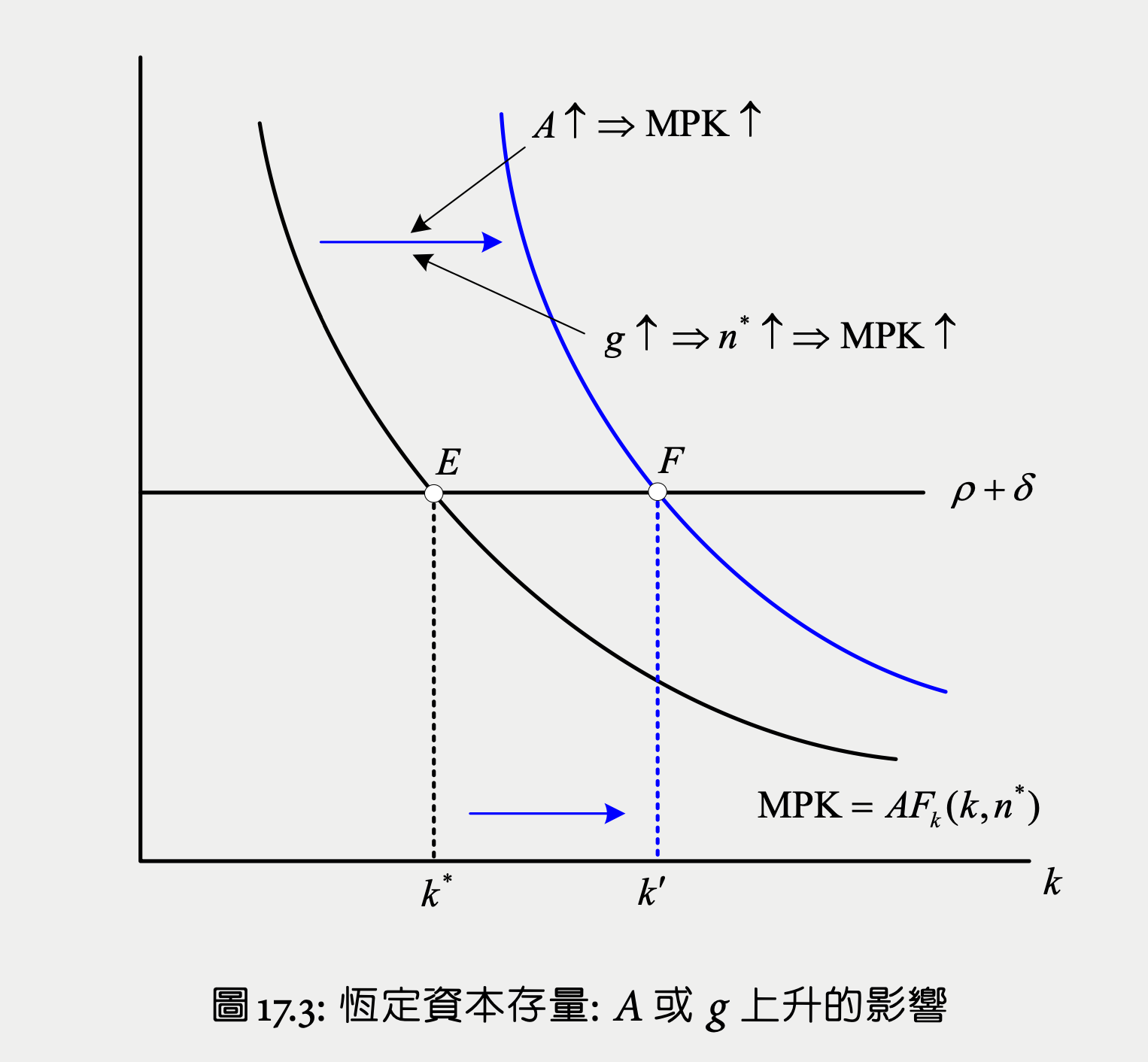
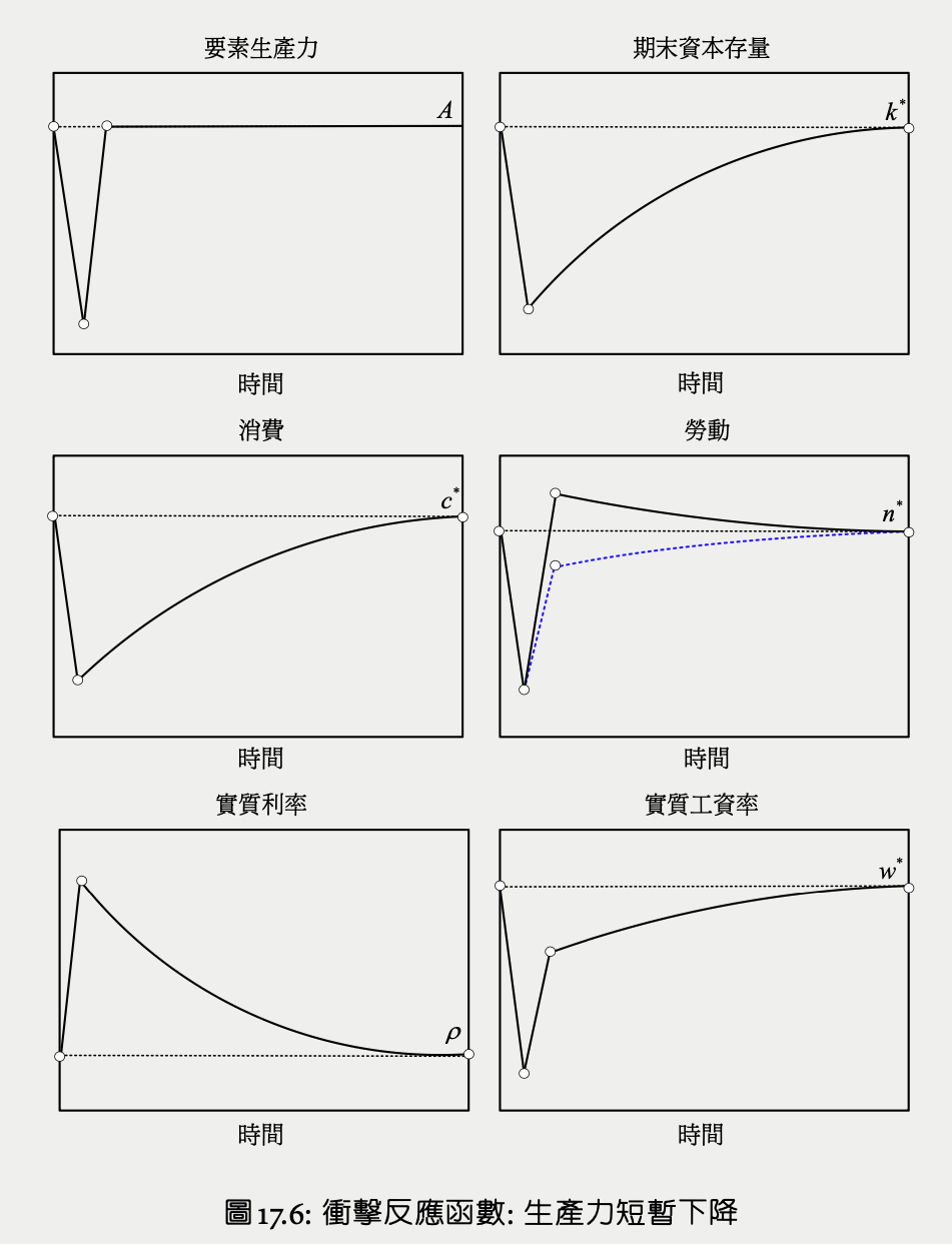
total factor productivity short-term down
during the shock
direct effect: \(y^s\) E -> D under the same interest rate & \(n^d\) shifts left
- output down -> non-labor income down, but only in that period, so the income effect i.e. the change in \(c^d\) & \(n^s\) can be ignored
- (under original interest rate) future \(A\) no change -> investment no change
- overall consumption demand no change
\(y^s\) D -> F & \(n^s\) shifts right
- short-term income down -> saving down (consumption smoothing) -> bonds market supply > demand -> interest rate up
- intertemporal substitution effect: \(r\) up -> \(n^s\) shifts right -> \(y^s\) upxz
\(c^d\) E -> F: \(r\) up -> \(c^d\) down
If it's #Ch13 廠商的投資決策 Ramsey Model, since the labor supply curve is static, \(A_t\) down will make the new equilibrium be B, a much bigger increase in \(r\) and decrease in \(c^d\). Meaning the dynamic labor supply smoothes the effect of shocks.
In theory, the overall change of labor depends, but in empirical studies, it will decrease.
- intertemporal substitution effect from interest rate increase is small -> \(n^s\) only shifts right a little
- the elasticity of labor supply to wage is high -> \(n^s\) is relatively flat
the entire curve
total productivity factor back up ->
- product market supply > demand i.e. bonds market demand > supply -> interest rate down -> labor supply down (intertemporal SE)
- wage = MPL up -> labor supply up (SE)
- intertemporal SE > SE -> black curve
- SE > intertemporal SE -> blue curve
total factor productivity permanently down
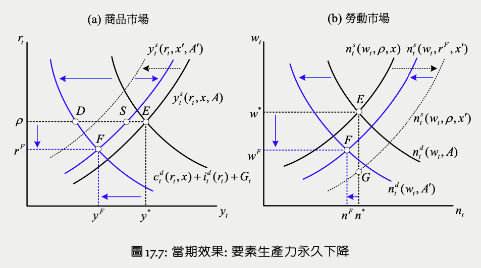
\(y^s\) E -> S
- direct effect: \(y^s\) & \(n^d\) shifts left
- income effect: \(y^s\) & \(n^s\) shifts right
- direct effect > income effect on \(y^s\) so overall still shifts left
- smaller overall product supply reduction due to more significant income effect
\(c^d\) shifts left a lot
- future MPK down -> desired capital stock down -> firm investment demand down
- future capital down -> future output down -> lifetime wealth down even more -> consumption demand down hugely
- future income reduction > current income reduction -> savings up for consumption smoothing
- \(|\Delta c^d_t|>|\Delta y^s_t|=ES\) -> commodity market supply > demand, bonds market demand > supply -> interest rate down
interest rate down -> (intertemporal SE)
- product supply down S -> F
- consumption demand up D ->
- \(n^s\) shifts left
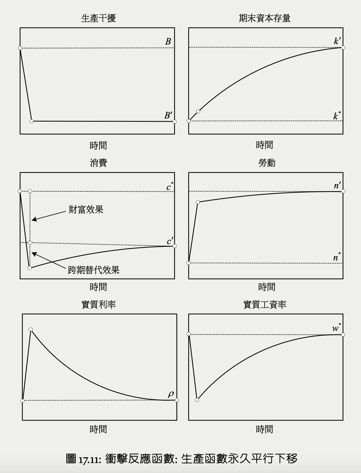
production surve shifts left
product supply surve shifts left horizontally
\(y=F(k,n)+B\), B down
steady-state
- direct effect: output down
- income effect: steady-state labor up, consumption down -> MPL down
- steady-state labor up -> MPK up -> desired capital stock up -> MPL up
- output is constant return to scale -> MPL changes cancelled -> MPL no change
- labor & capital up -> output up
- overall output depends
short-term
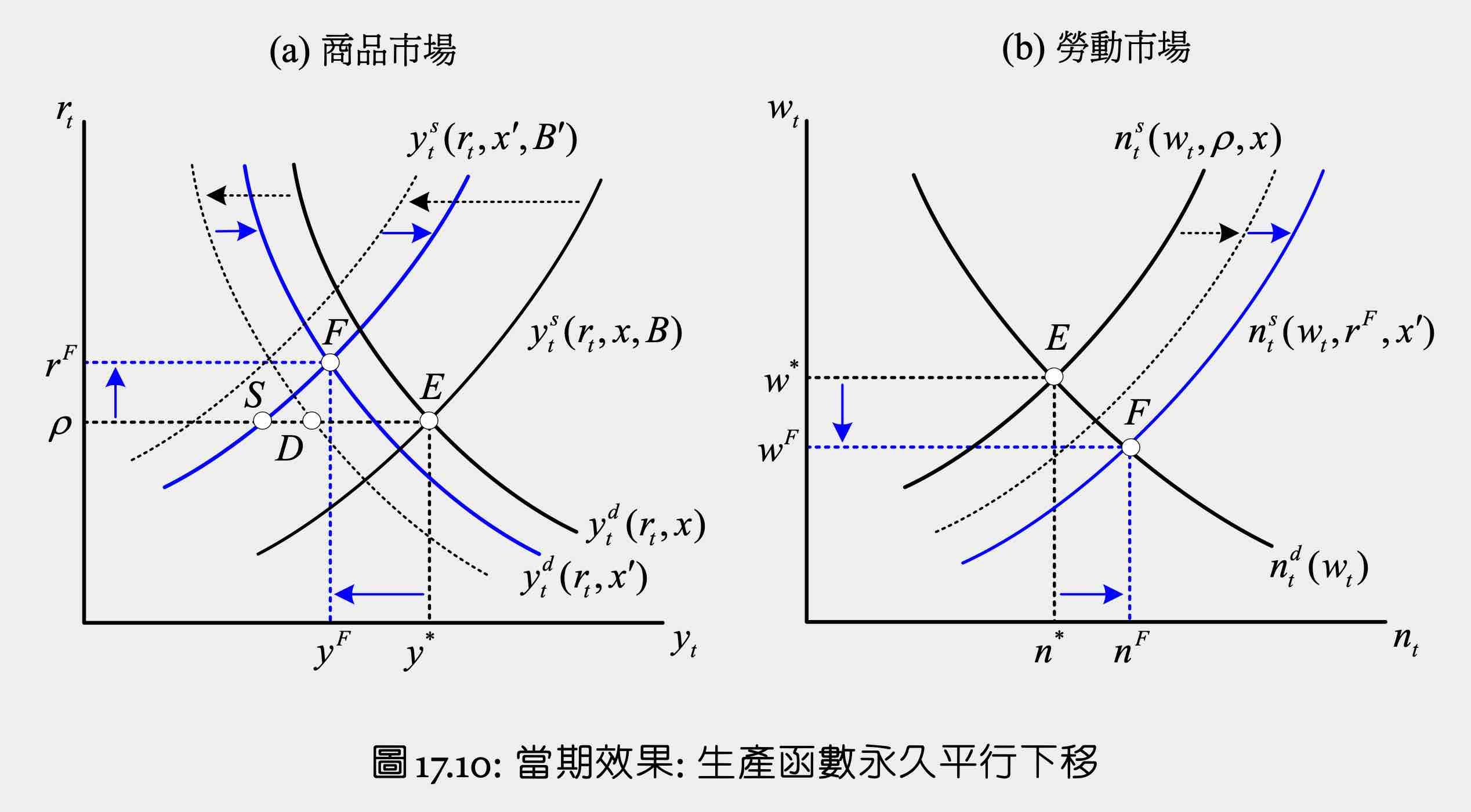
E -> S
- direct effect: commodity supply shifts left
- income effect
- steady-state labor up -> MPK up -> desired capital stock up -> lifetime wealth not down by too much
- labor supply shifts right a bit -> commodity supply shifts right a bit
- consumption demand shifts left a bit E -> D < E -> S
for firm
- steady-state labor up -> MPK up -> desired capital stock up -> investment up -> commodity demand shifts right from D
commodity market demand > supply, bonds market supply > demand -> interest rate up
labor market
- labor demand not affected
- lifetime wealth down -> labor supply shifts right
- interest rate up -> labor supply shifts right
- labor market supply > demand -> wage down
overall
- output down
- consumption down
- investment up
- labor up
- interest rate up
- wage down
the entire curve
Crusoe
available fruits permanently down ->
- working hour permanently up
- MPL (shadow wage) down
- MPK (shadow interest rate) up
- MPK up -> investment up
- consumption permanently down
- since capital hasn't changed in the short term, consumption magnificently down in the short term
- can view as the intertemporal SE of shadow interest rate up
- lifetime utility down
holding labor or capital constant
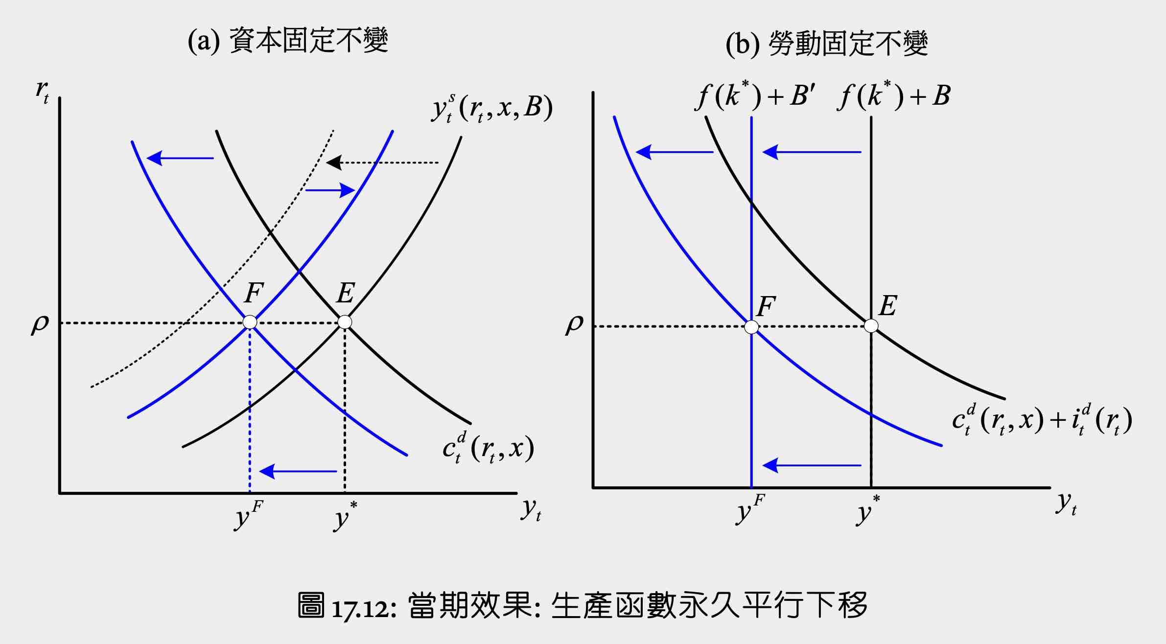
(a) capital is constant
capital can't be changed -> national saving = 0, each period is independent to another, all the external shocks are consumed in the same period
B -> down
- direct effect: output down -> \(y^s\) shifts left
- income effect: wealth down -> \(n^s\) shifts right, \(c^d\) shifts left -> \(y^s\) shifts right
\(y^s\) & \(c^d\) shifts left by the same magnitude
- output & consumption down by the same magnitude
- interest rate unchanged
- wage down
(b) labor is constant #Ch13 廠商的投資決策 Ramsey Model
labor can't be changed -> \(n^s\) not affected by \(r\) -> vertical curve
B -> down
- direct effect: output down -> \(y^s\) shifts left
- income effect: wealth down -> \(c^d\) shifts left
labor constant -> MPK won't be changed -> desired capital stock unchanged -> investment unchanged
- output & consumption down by the same magnitude
- interest rate unchanged
Ch18 Monetary Policy Analysis of RBC Model
effect of government purchase short-term increase
commodity market & labor market
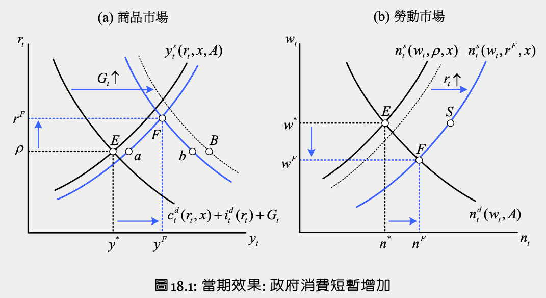
bonds market
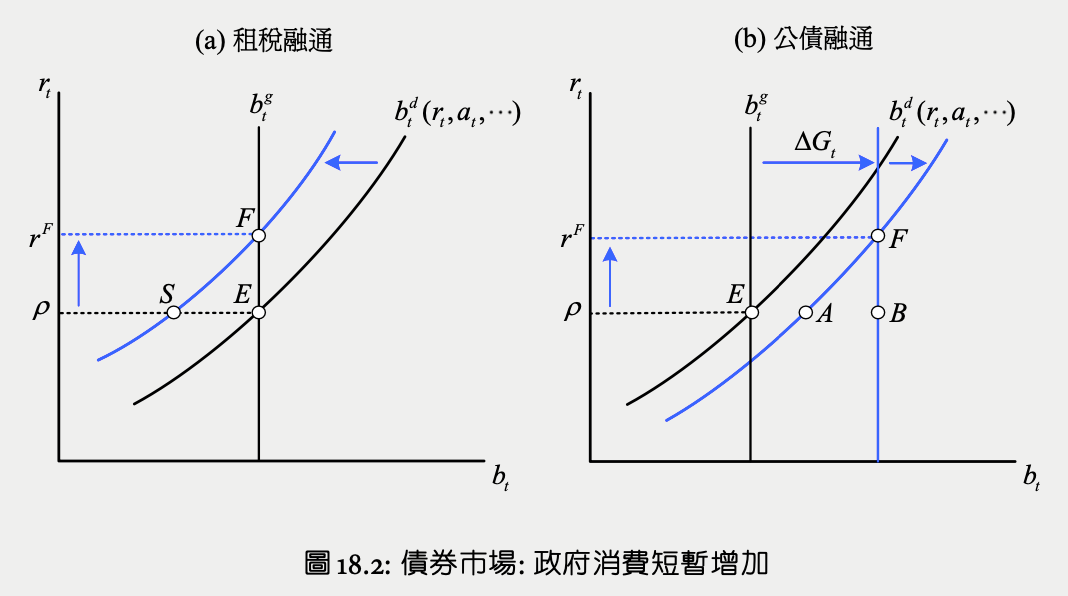
- direct effect: commodity demand E -> B
- income effect: labor supply shifts right a bit, consumption demand shifts left a bit B -> b-> commodity supply shifts right a bit E -> a
- the change to lifetime wealth is very small, so the income effect is very small, basically negligible
commodity market supply > demand, bonds market demand > supply -> interest rate up -> intertemporal SE:
- private consumption & firm investment down -> \(c^d\) b -> F
- labor supply up -> \(y^s\) a -> F
overall
- real interest rate up
- output up
- private consumption down
- firm investment down
same as #Ch13 廠商的投資決策 Ramsey Model except output change as labor supply is fixed in Ramsey Model
The result is the same whether the government funds the purchase through lump-sum tax or bonds.
- lump-sum tax
- current wealth down -> saving demand down -> bonds market supply > demand -> interest rate up
- bonds
- future wealth down -> saving demand up, but government bonds supply up more -> bonds market supply > demand -> interest rate up
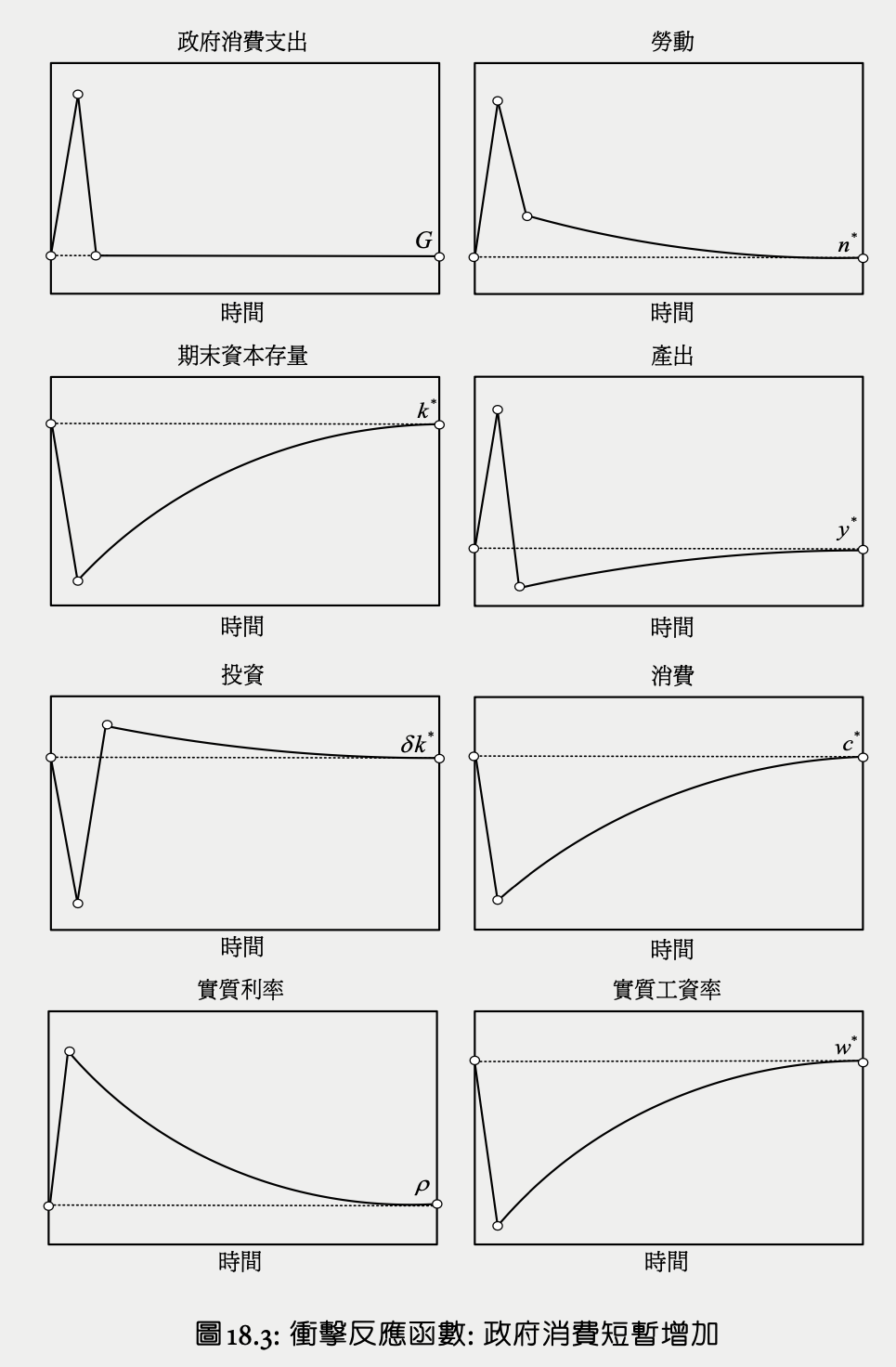
analysis
- crowding effect
- private consumption & firm investment down
- output increase EF < government purchase increase EB i.e. \(\dfrac{\Delta y_t}{\Delta G_t}<1\)
- the multiplier effect is non-existent
- \(\Delta y_t\) is bigger in #Ch7 靜態模型的均衡分析#政府消費支出增加 since there's no consumption smoothing when bonds can't be buy (ref: Bruno Fernandez)
- \(\Delta y_t=0\) in #Ch13 廠商的投資決策 Ramsey Model since labor supply if fixed, meaning government purchase crowds out all private consumption & investment
- social welfare
- increasing government purchase will make output i.e. GDP increase, but at the cost of social welfare i.e. private utility
- consumption down, labor up, wage down -> current utility down
- firm investment down -> future output down -> future consumption down -> future utility down
- however, the model leaves out the fact that government purchases have externality irl
- government purchase is not the determining force to economic fluctuations
- empirical data: GDP \(\propto\) \(1/r\), GDP \(\propto C, I, w\)
- RBC analysis of government purchase up: GDP \(\propto\) \(r\), GDP \(\propto 1/C, 1/I, 1/w\)
effect of government purchase permanent increase
Steady-state
See #Ch17 Real Business Cycle RBC Model#effect of government consumption change
Short-term
Similar to #Ch17 Real Business Cycle RBC Model#production surve shifts left
assumge government purchase up EB, funded with lump-sum tax
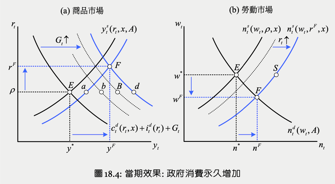
under original interest rate
- direct effect
- \(c^d\) E -> B
- current wealth down EB
- income effect: \(n^s\) shifts right, \(c^d\) shifts left from B -> \(y^s\) shifts right E -> a -> current wealth up Ea
- current wealth down aB
- steady-state output up -> future income up -> \(\Delta\) lifetime wealth < aB -> \(c^d\) shifts left B -> b < B -> a
- commodity market demand - supply = ab
- steady-state labor up -> MPL up -> desired capital stock up -> firm investment demand up -> \(c^d\) shifts right b -> d
- commodity market demand - supply = ad -> interest rate up
interest rate up
- private consumption & firm investment demand down -> \(c^d\) d -> F
- does not cancel out the previous firm investment up
- labor supply up -> \(y^s\) a -> F
overall
- output up
- interest rate up
- private consumption down
- firm investment up
- \(\mathrm{MPK}_{t+1}-\delta=r_t\)
- \(MPK_{t+1}\) up -> money flow from bonds to capital -> \(r_t\) up
- so the capital decrease from \(r_t\) up will not cancel out the capital increase
- wage down
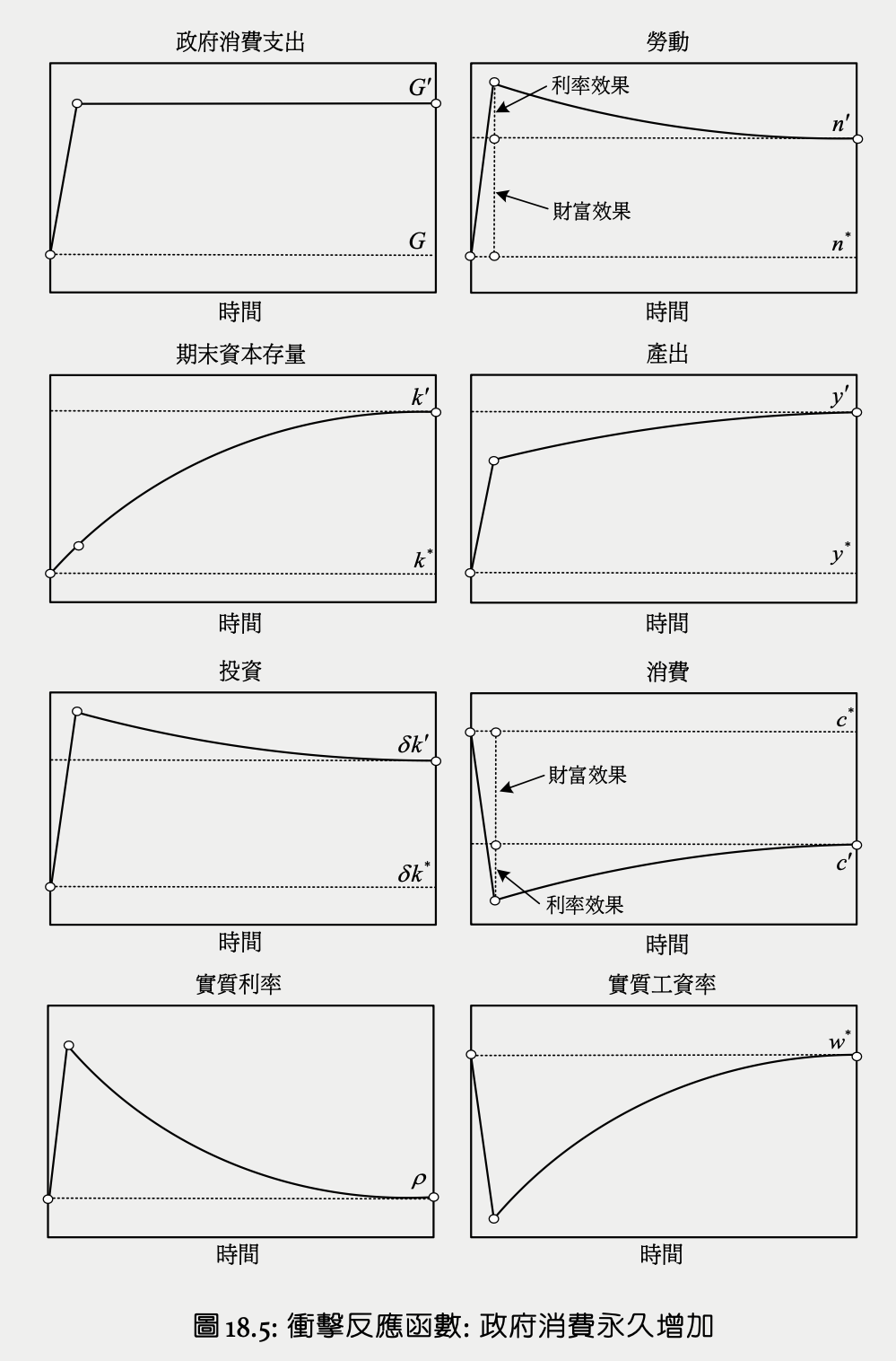
tax
government expenditure & total factor productivity is irrelevant so let \(G_t=0\), \(A_t=1\)
government budget constraint
- tax \(\tau^c\) of private consumption
- tax \(\tau^n\) of consumer labor income
- tax \(\tau^k\) of firm profit
- transfer payment \(v_t\) to consumer
since all the tax are transferred back to consumers ultimately, there's no income effect but only substitution effect
firm profit tax = tax from income from capital
so firm's profit = the income from capital
consumer budget constraint
where \(a_t=d_t+v_t\)
consumer optimization problem
ccontemporaneous SE
intertemporal SE
no \(\tau^c\)
firm optimization problem
- \(y_t=F(k_{t-1},n_t)\)
- \(i_t=k_t-(1-\delta)k_{t-1}\)
general equilibrium
steady-state
example
- \(u(c,l)=\ln c+\ln l\)
- \(y=k^\alpha n^{1-\alpha}\)
where \(\phi=\dfrac{\alpha}{\rho+\delta}\)
there's a ratio \((1-\tau^k)\phi\in(0,1)\) between \(k^*\) & \(y^*\)
with \(c^*+\delta k^*=y^*\)
be aware not to directly \(w^*=\dfrac{\partial y^*}{\partial n^*}\) because it makes no sense, they are numerical values
effect of \(\tau^n\) or \(\tau^c\) up
- \(\tau^n\) or \(\tau^c\) up -> \(n^*\) down -> \(y^*\) & \(k^*\) down
- lifetime wealth not changed but steady-state income is still changed
- \(\dfrac{y^*}{n^*}\) = constant (since \(\tau^k\) unchanged) so MPL & \(w^*\) unchanged
- post-tax wage down
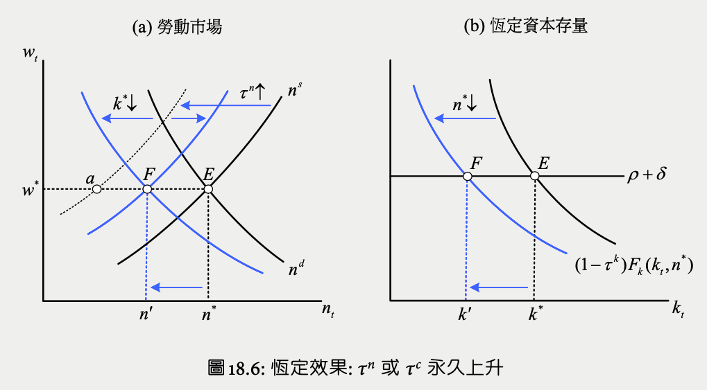
effect of \(\tau^k\) up
- \(\tau^k\) up -> \(n^*\) down -> \(y^*\) down -> \(k^*\) down -> MPL & \(w^*\) down
- \(\dfrac{y^*}{n^*}=[(1-\tau^k)\phi]^{\alpha/(1-\alpha)}\) down, meaning \(y^*\) down more than \(n^*\)
- \(\dfrac{k^*}{y^*}=(1-\tau^k)\phi\) down, meaning \(k^*\) down more than \(y^*\)
- \(\dfrac{d\ln c^*}{d \tau^k}<0\) -> \(c^*\) down
- can't be derived with intuition since \(c^*+\delta k^*=y^*\) and \(\Delta k^*>\Delta y^*>\Delta n^*\)
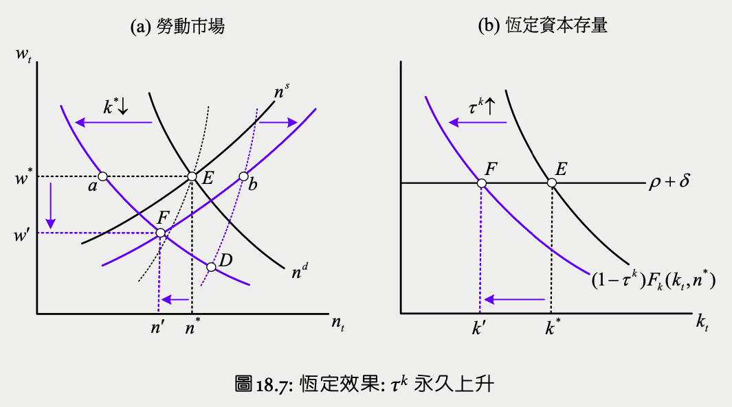
一例一休
set HUGE overtime pay i.e. wage higher when labor hour > max labor hours
output & profit curve
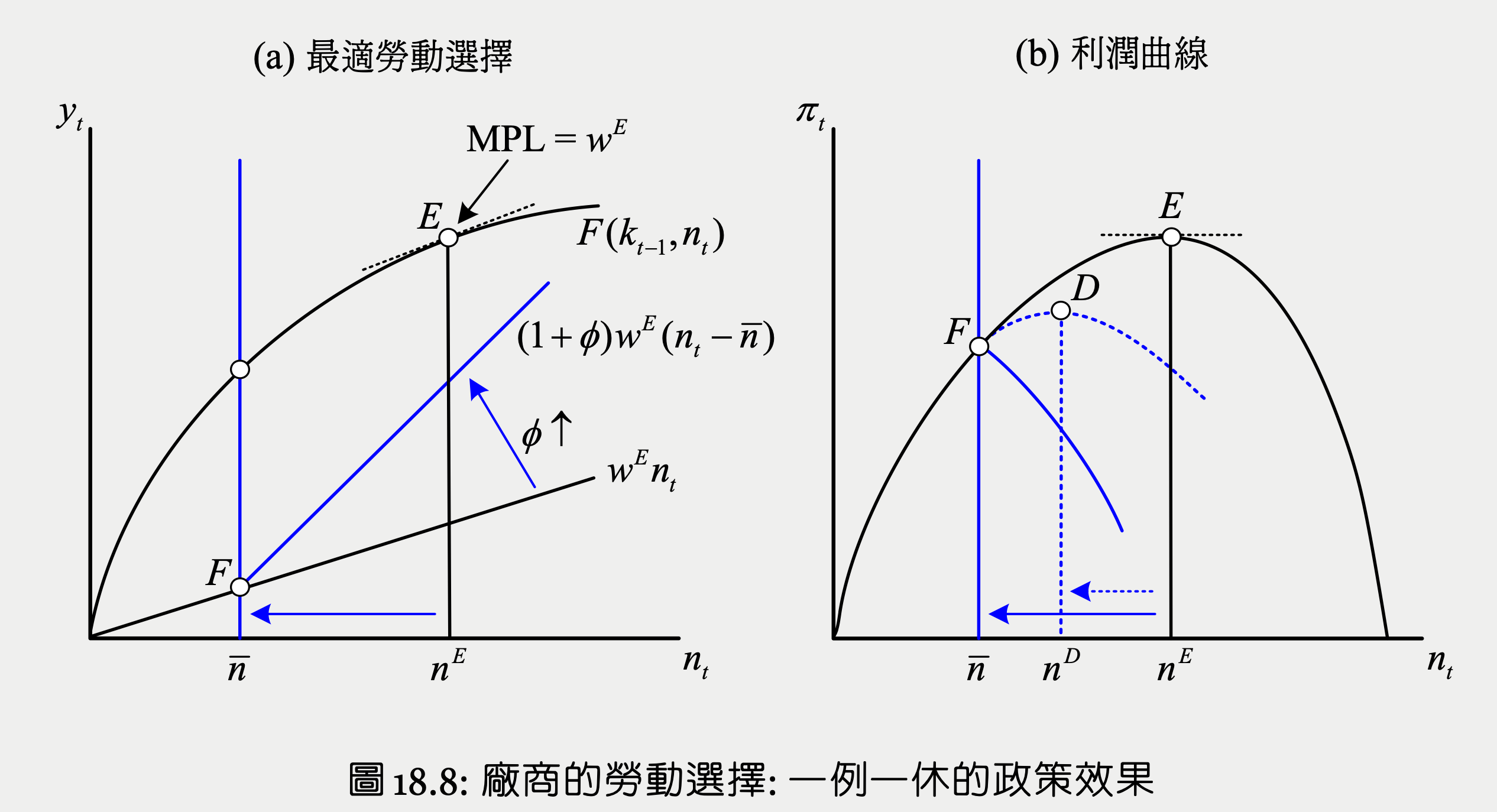
wage higher when \(n_t>\bar{n}\) -> profit vs. labor curve of \(n_t>\bar{n}\) changes
- moderate overtime pay -> dotted blue line -> \(\bar{n}<n^D<n^E\) optimal point
- huge overtime pay -> blue line -> \(\bar{n}\) optimal point
labor demand curve
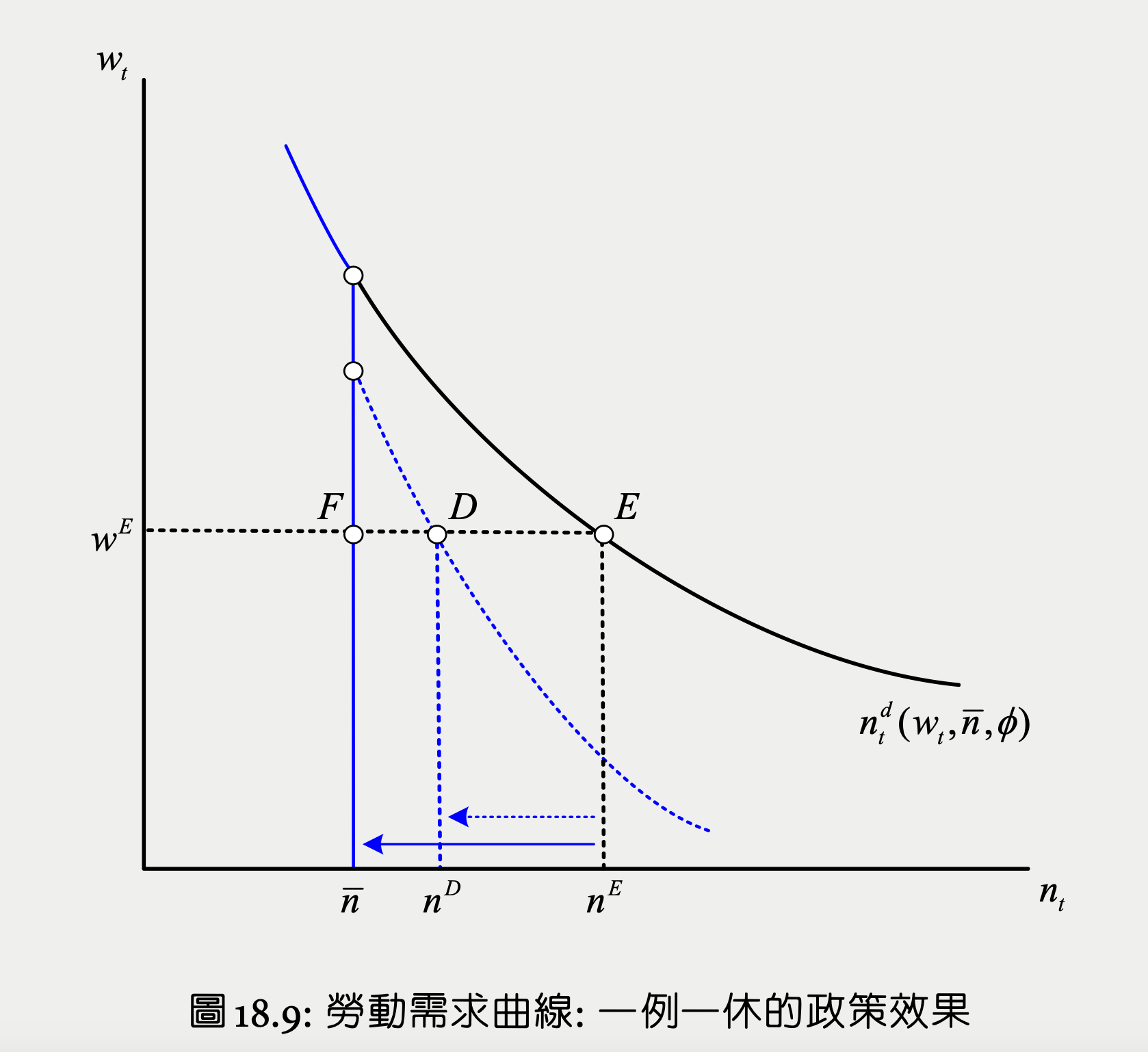
- moderate overtime pay -> dotted blue line, labor demand steeper, smaller elasticity to wage
- huge overtime pay -> blue line -> \(\bar{n}\) optimal point, labor demand vertical, independent of wage
- which is the case in 一例一休
labor supply curve
no income effect to the whole economy
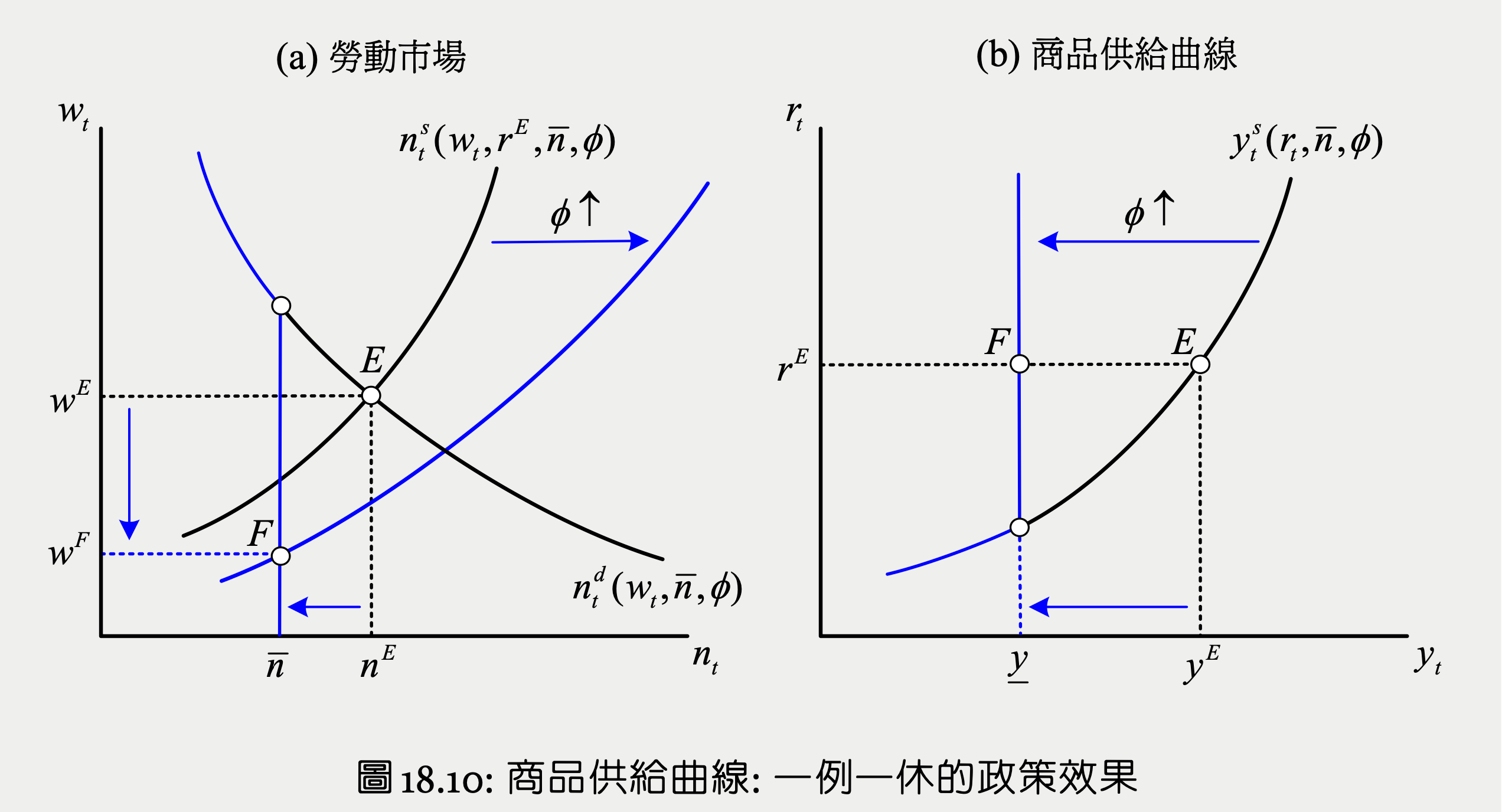
- SE: overtime pay up -> labor supply flatter in \(n_t>\bar{n}\), more elastic to wage
- labor demand vertical -> equilibrium labor down -> output & income down
- IE: income down -> labor supply shifts right
- output inelastic to interest rate in \(y_t>\bar{y}\) due to vertical labor demand in \(n_t>\bar{n}\)
steady-state
- labor down -> MPK down -> desired capital down -> future output down, MPL down, labor further down
- labor market supply > demand -> wage down
- firm labor demand inelastic to wage -> labor absorbs 100% of the wage reduction