Statistics¶

Materials¶

Tables¶

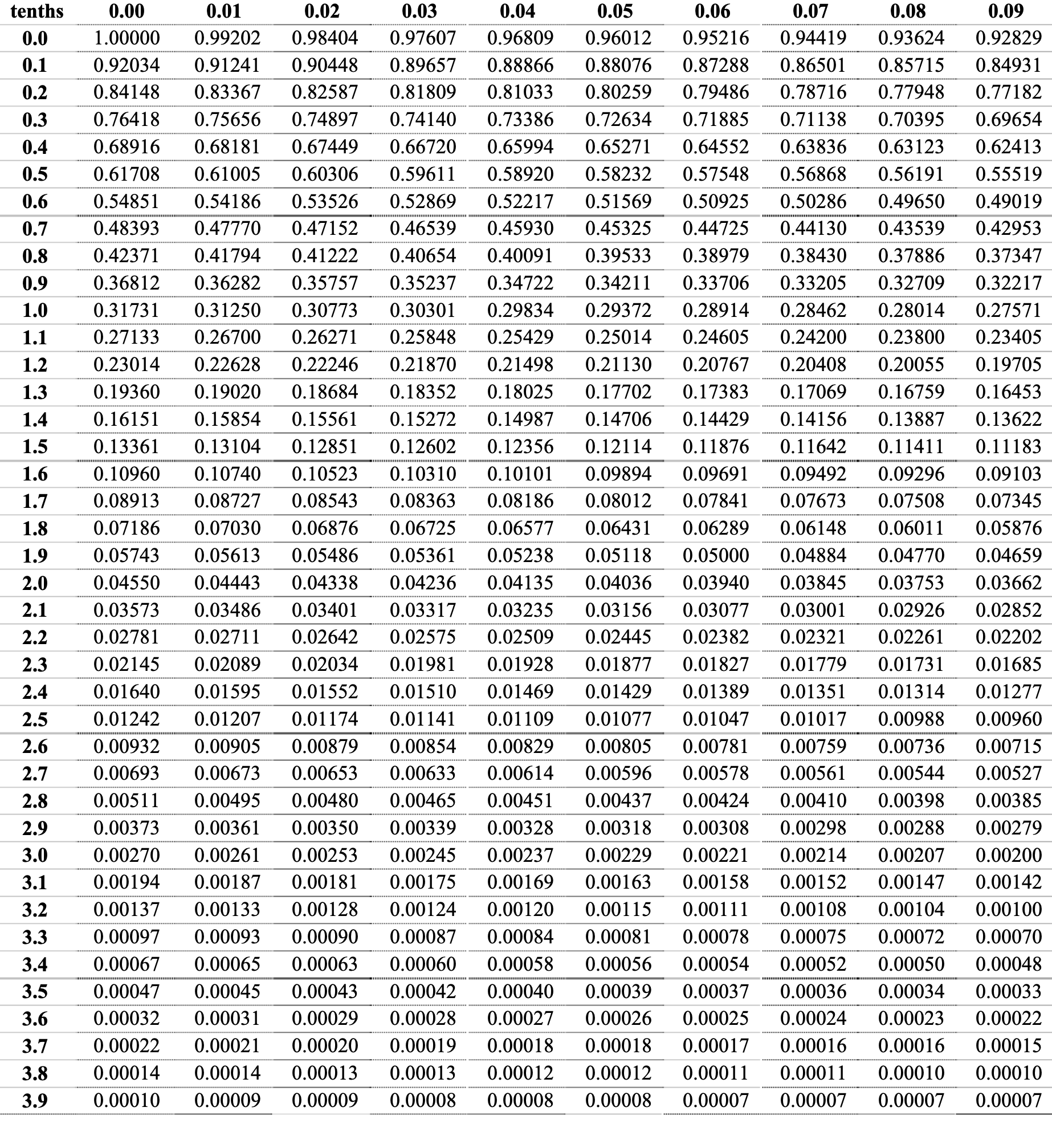
Z Table¶

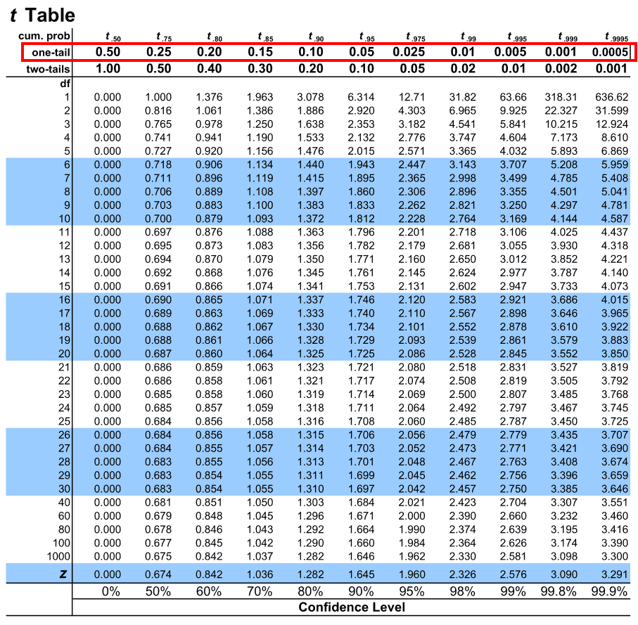
T Table¶

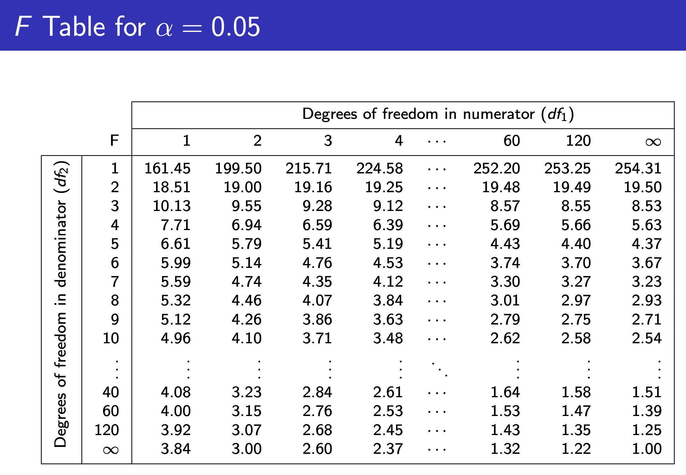
F Table¶

Notation¶

\(p\) = population
\(\hat{p}\) = sample

Intro¶

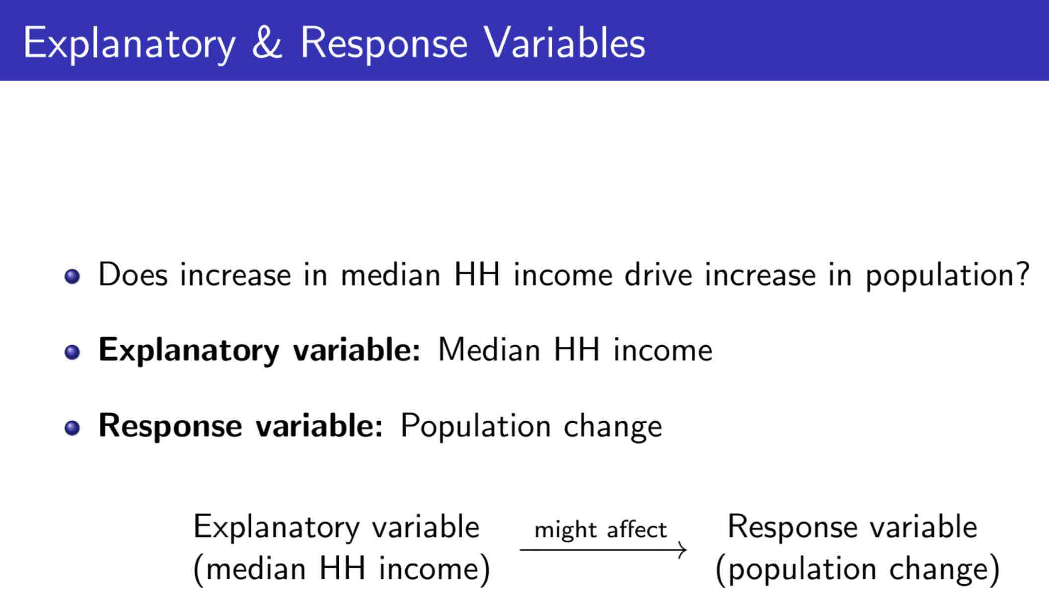
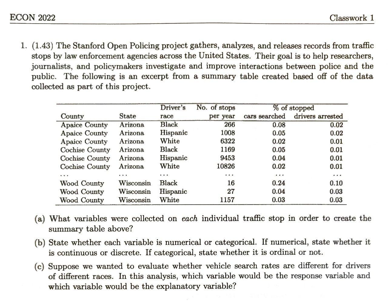
Explanatory & Response variable¶

func (explanatory) response

Variables¶

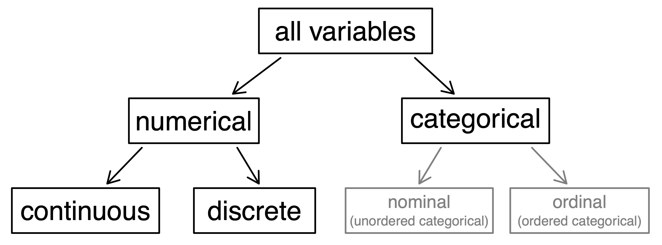
numeric
- discrete
- continious
categorical
- ordinal
  - can be sorted
  - e.g. A, B, C ...
- not ordinal

Sampling¶

simple random sampling
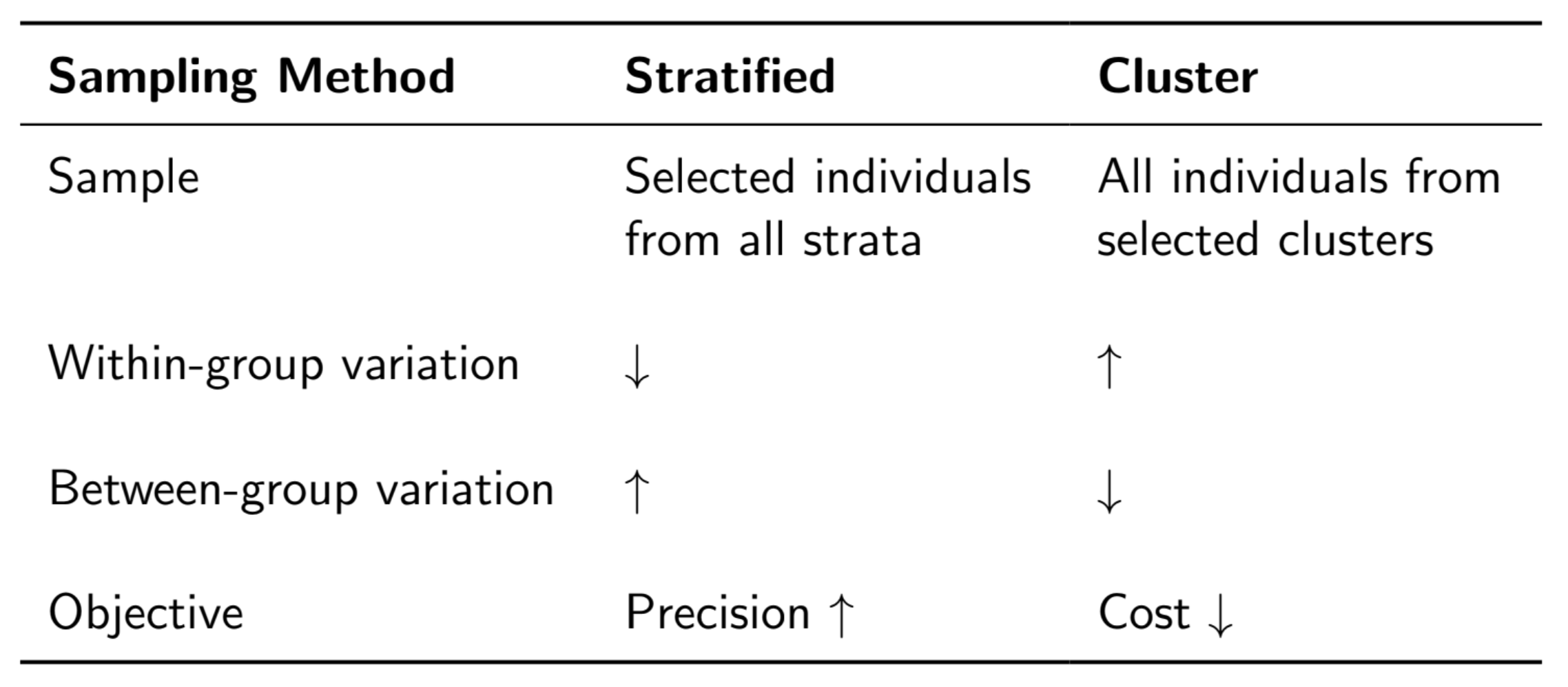
stratified sampling
- group into stratas -> sample within each strata (sample unit: case)
- each strata has its charactersitcs
cluster sampling
- divide into clusters -> sample clusters (sample unit: cluster)
multistage sampling
- divide into clusters -> sample clusters -> sample within each selected cluster

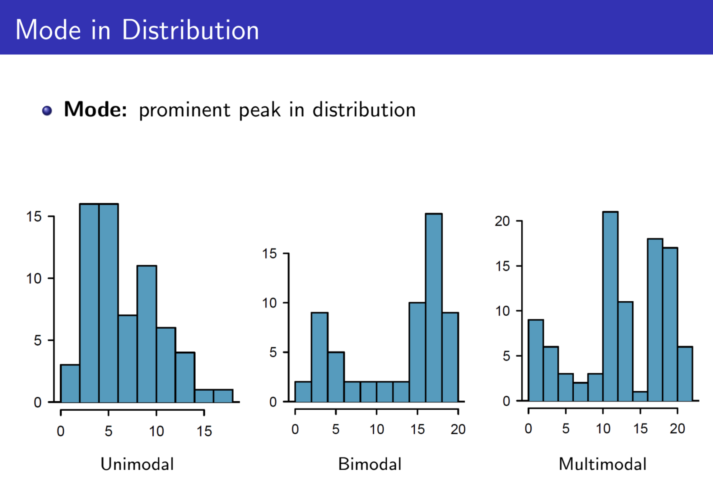
Distribution Mode¶

How are local maxima distributed?

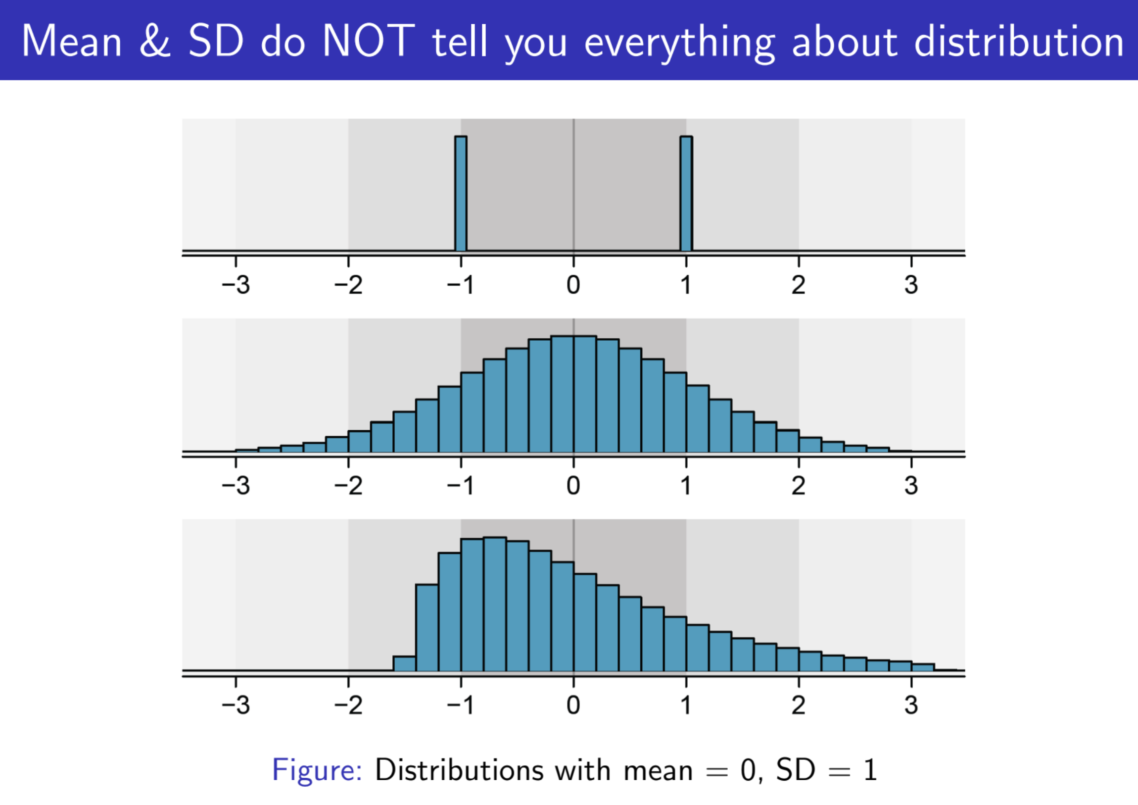
Mean & Variance¶

Same mean & variance may stem from very different distributions

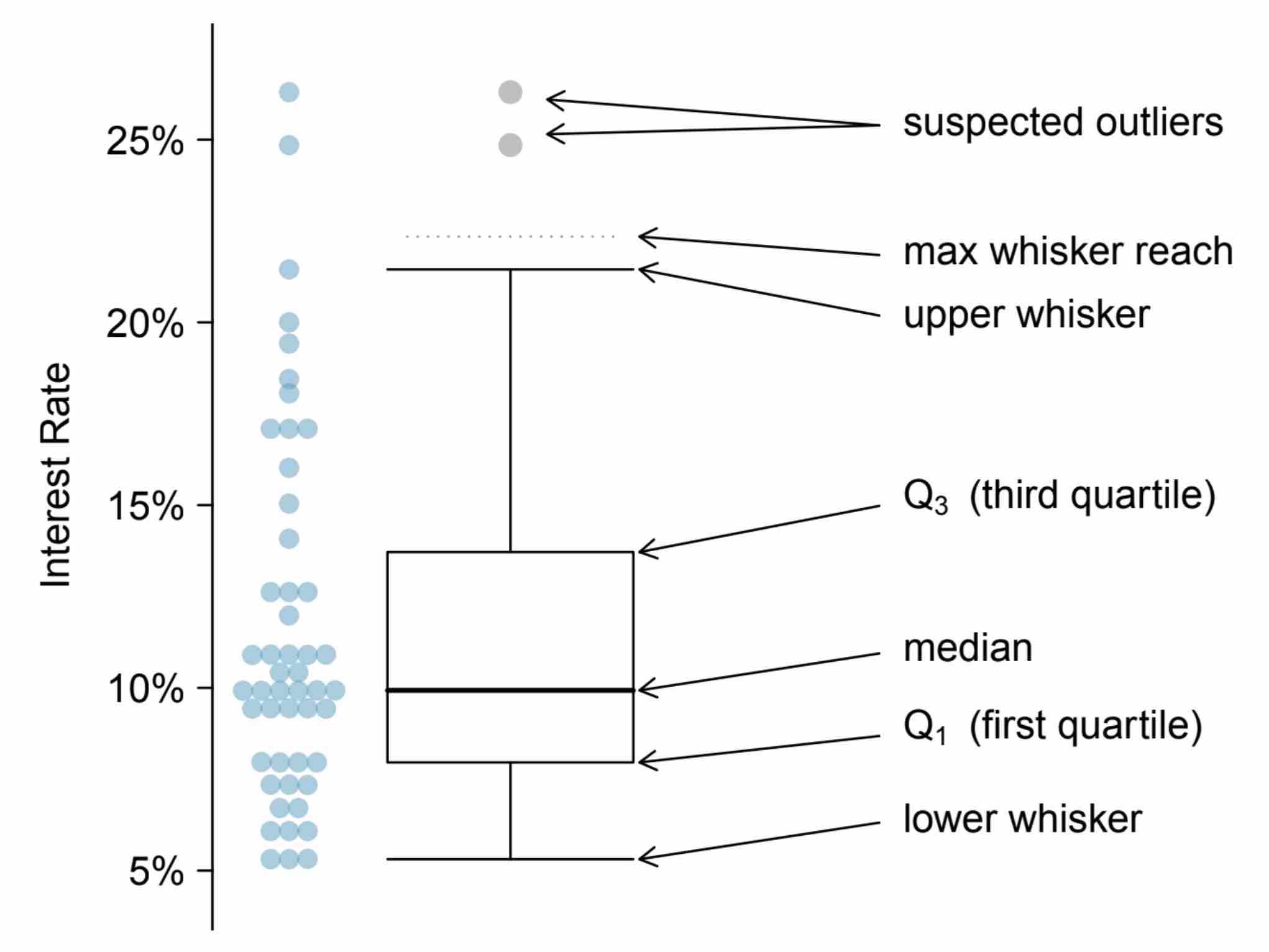
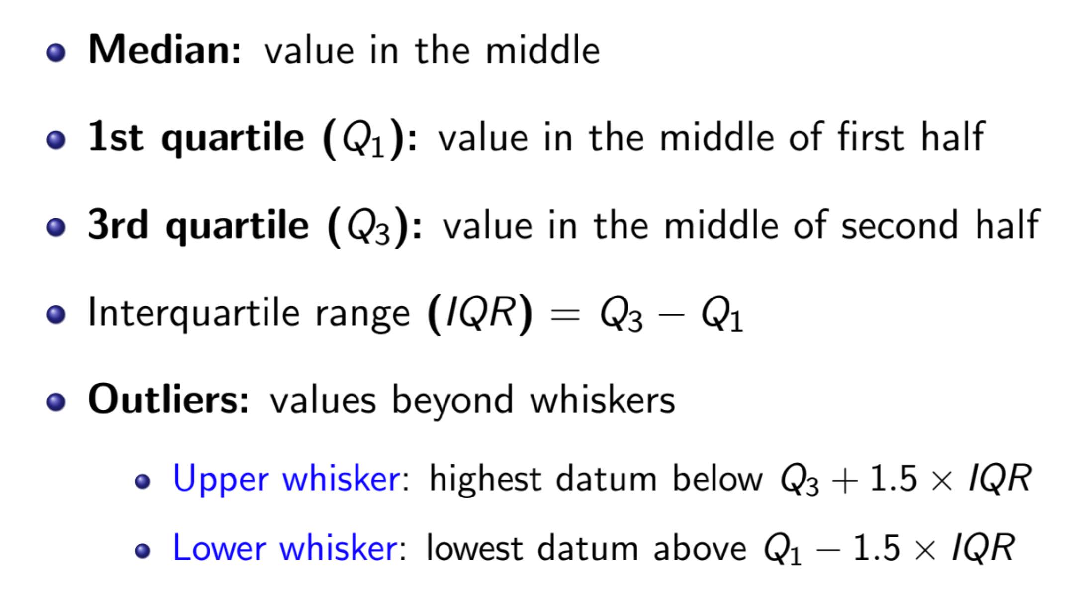
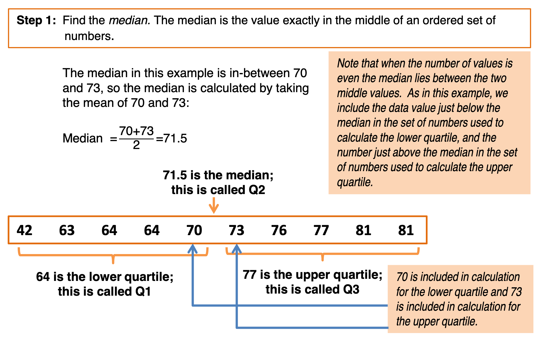
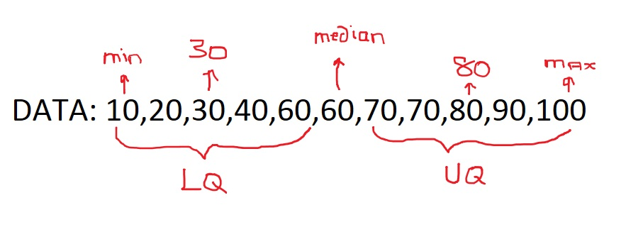
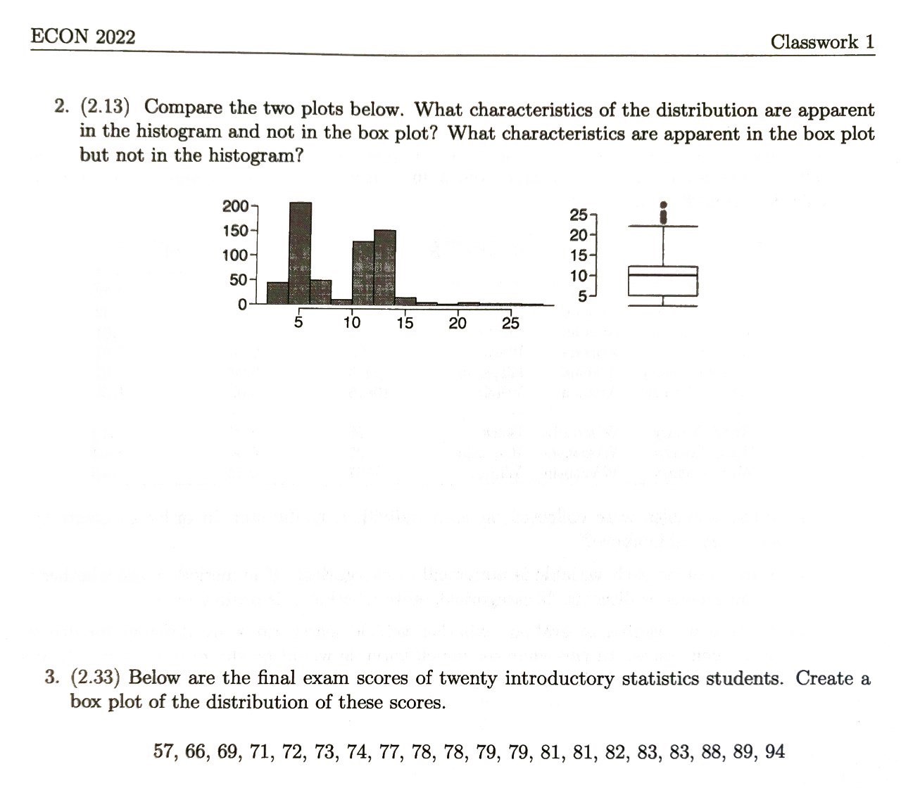
Box Plot¶

median = middle number
- 2 number -> average
Q1 = middle number in upper half
- median has 2 number -> middle between min & closest median
Q3 = middle number in lower half
IQR = Q3-Q1
upper whisker = min(max, Q3 + 1.5 x IQR)
lower whisker = max(min, Q1 - 1.5 x IQR)
outliers = those ouside of upper & lower whisker

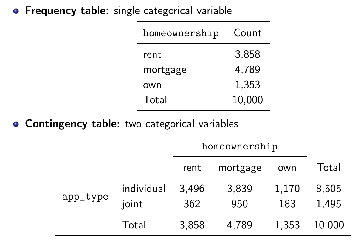
Tables¶

Frequency table
Contingency table

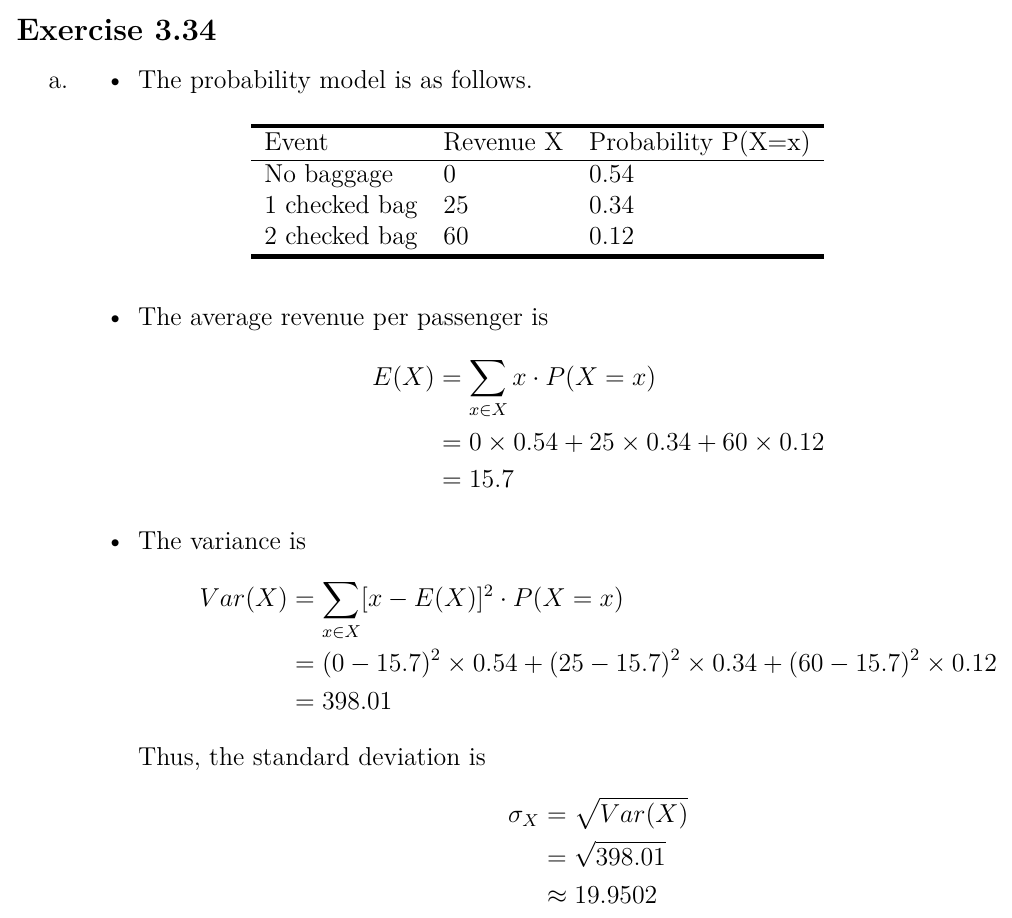
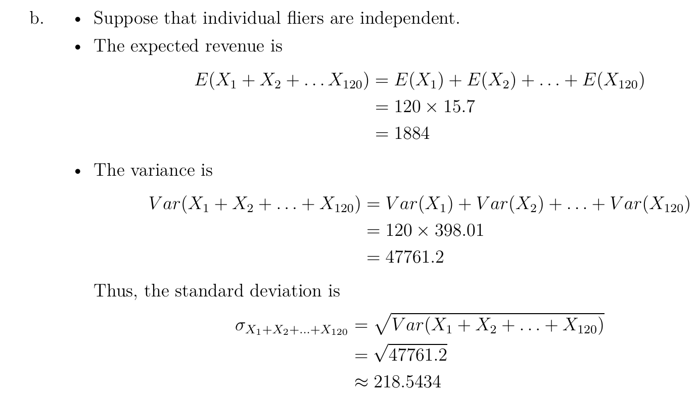
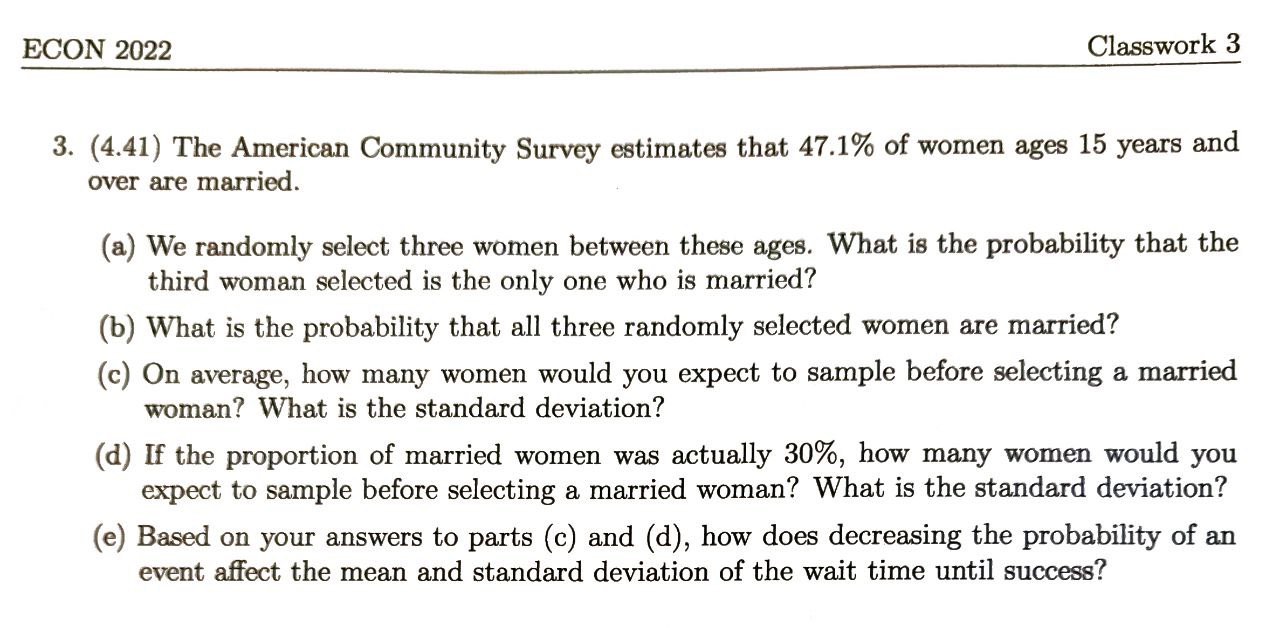
Problems¶

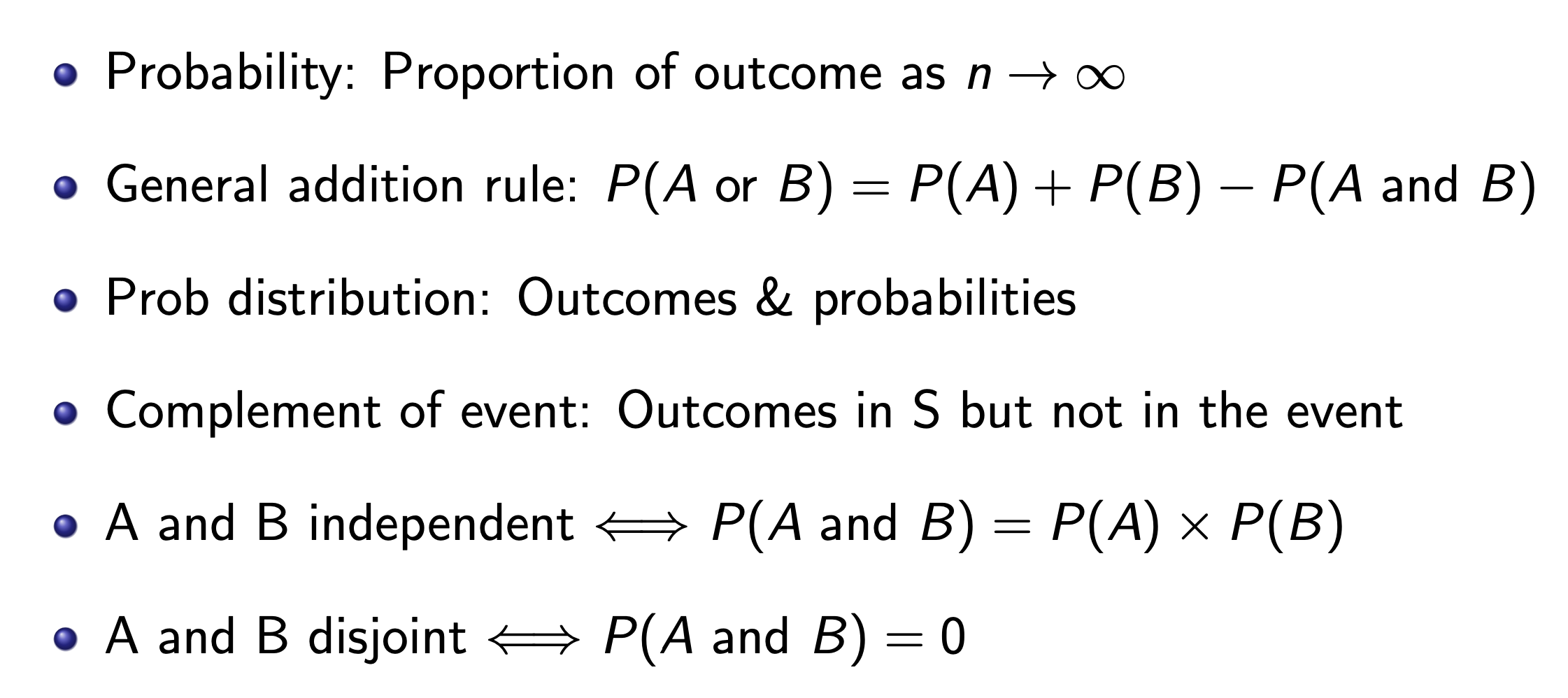
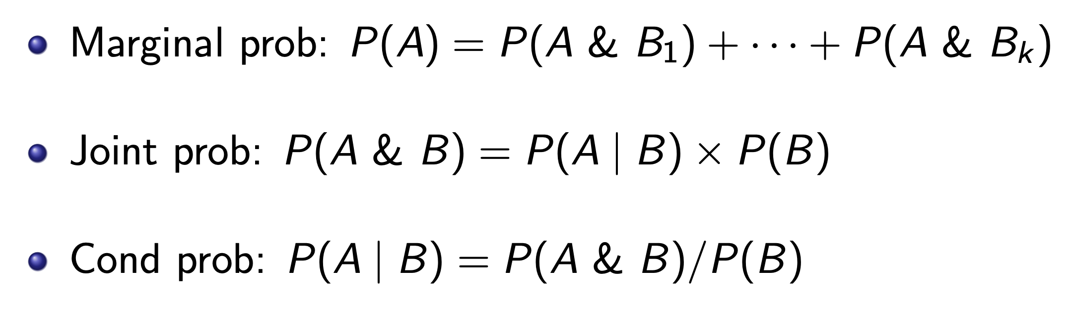
Probability¶

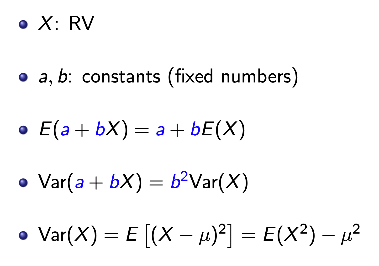
Random Variables¶

sample space -> number

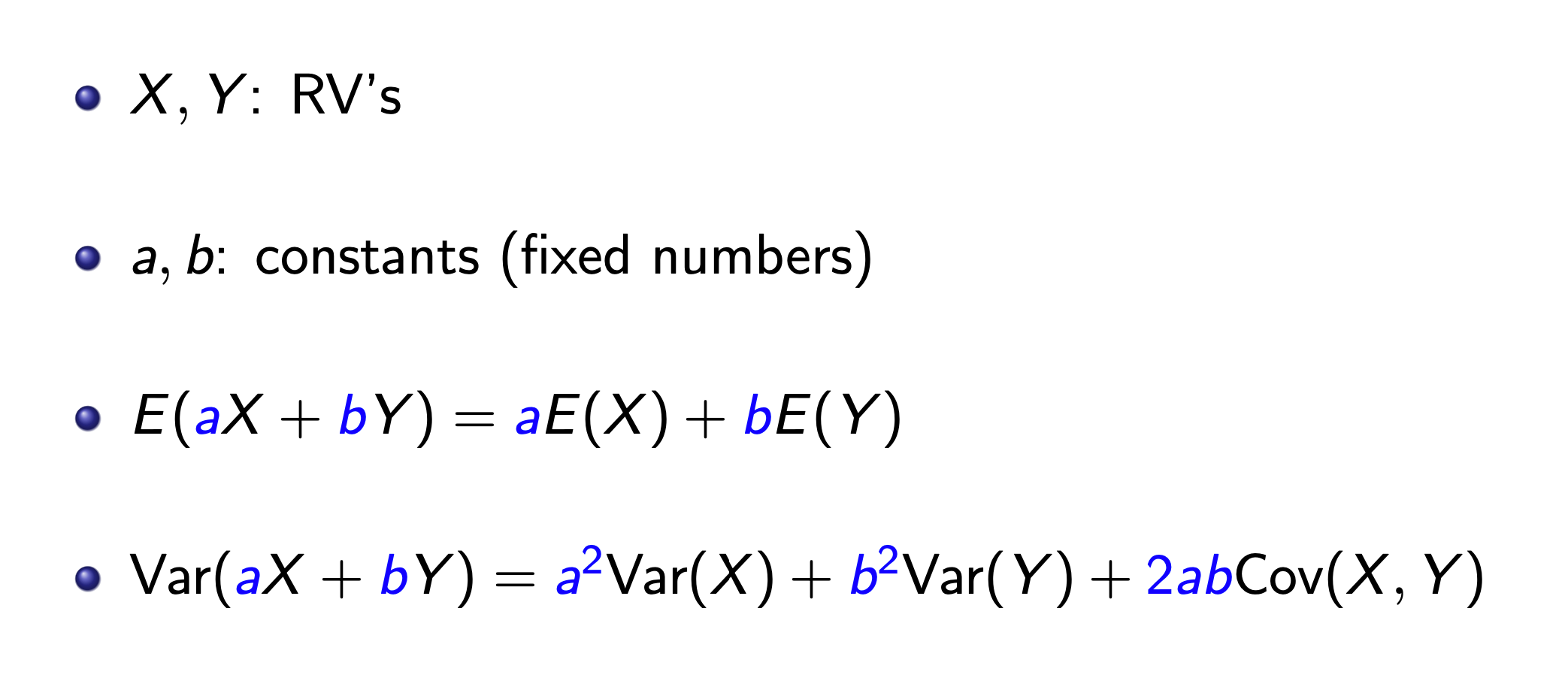
Rules¶

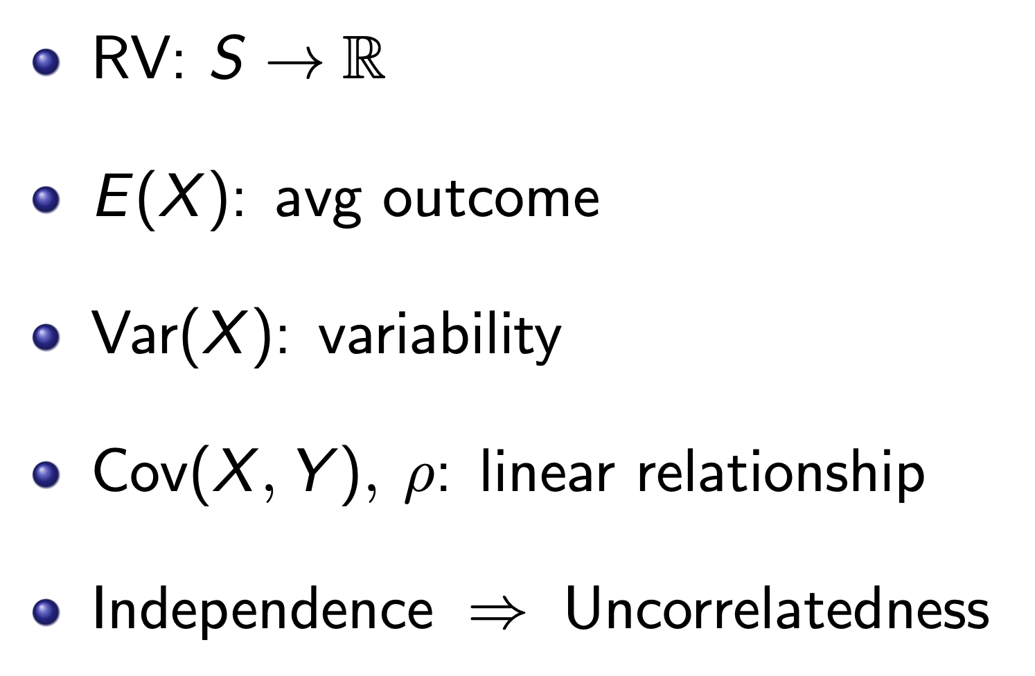
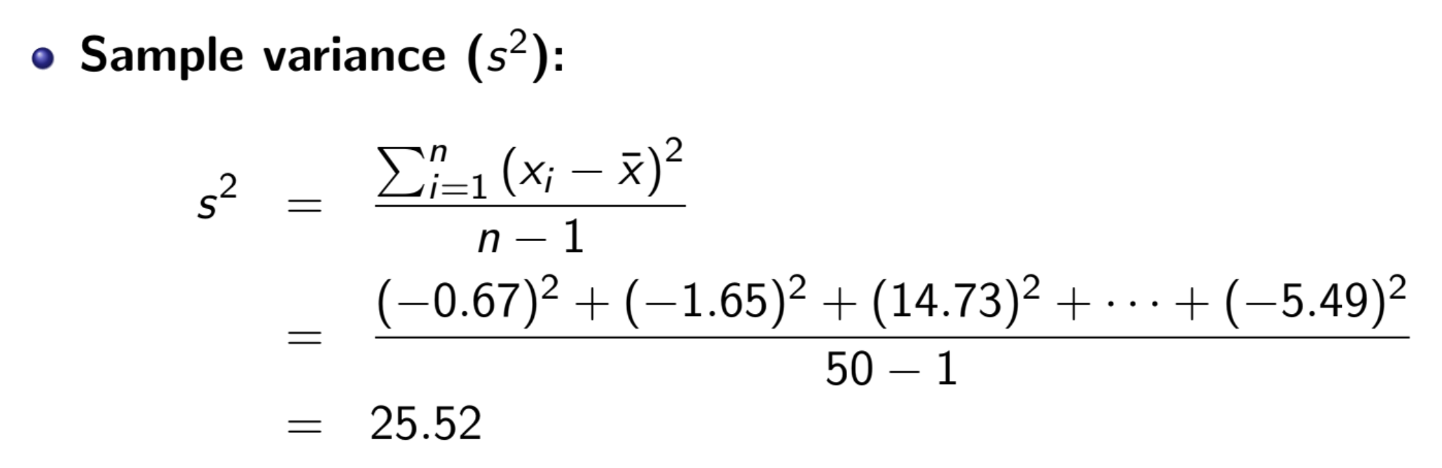
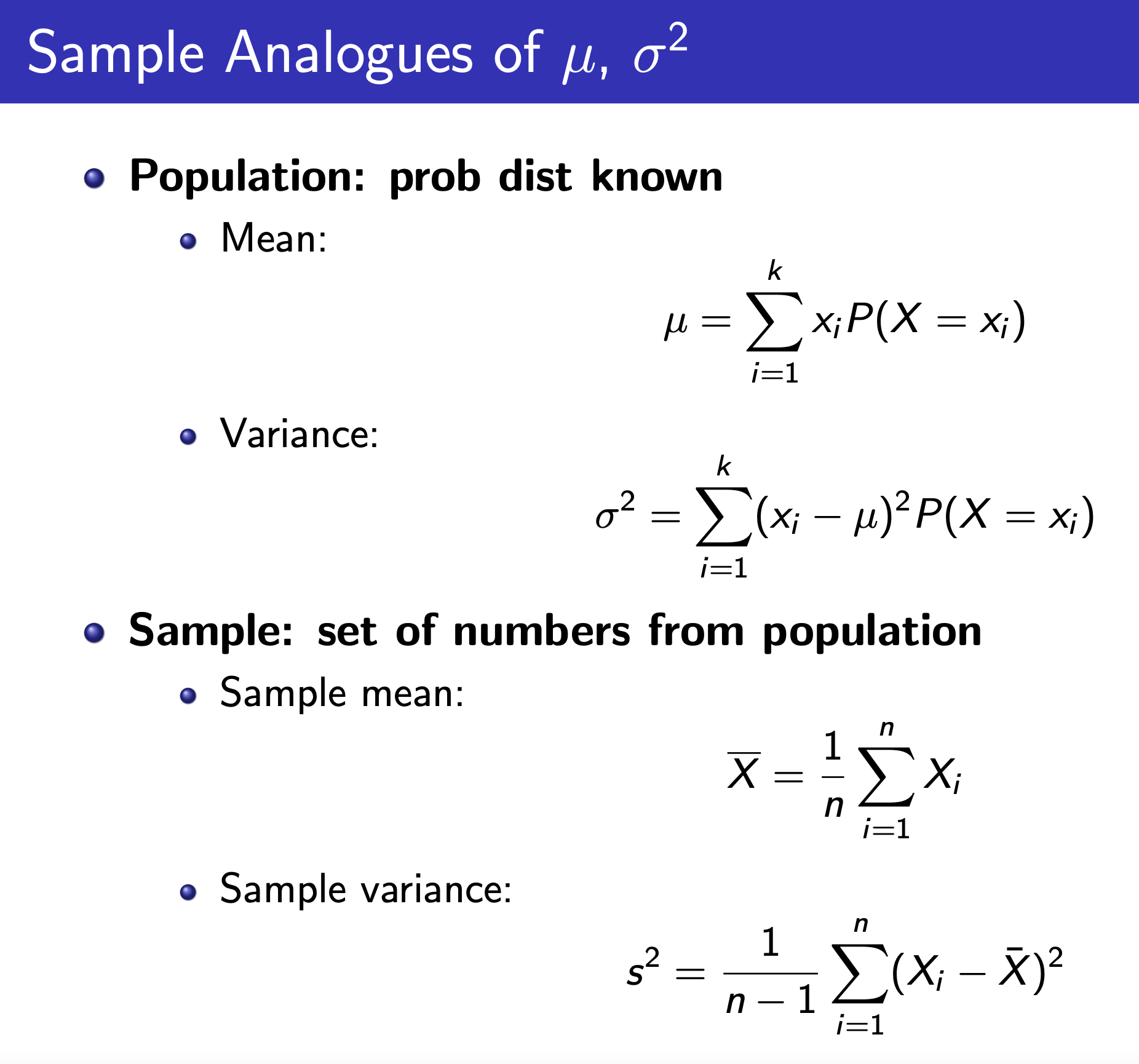
Variance vs. Sample Variance¶

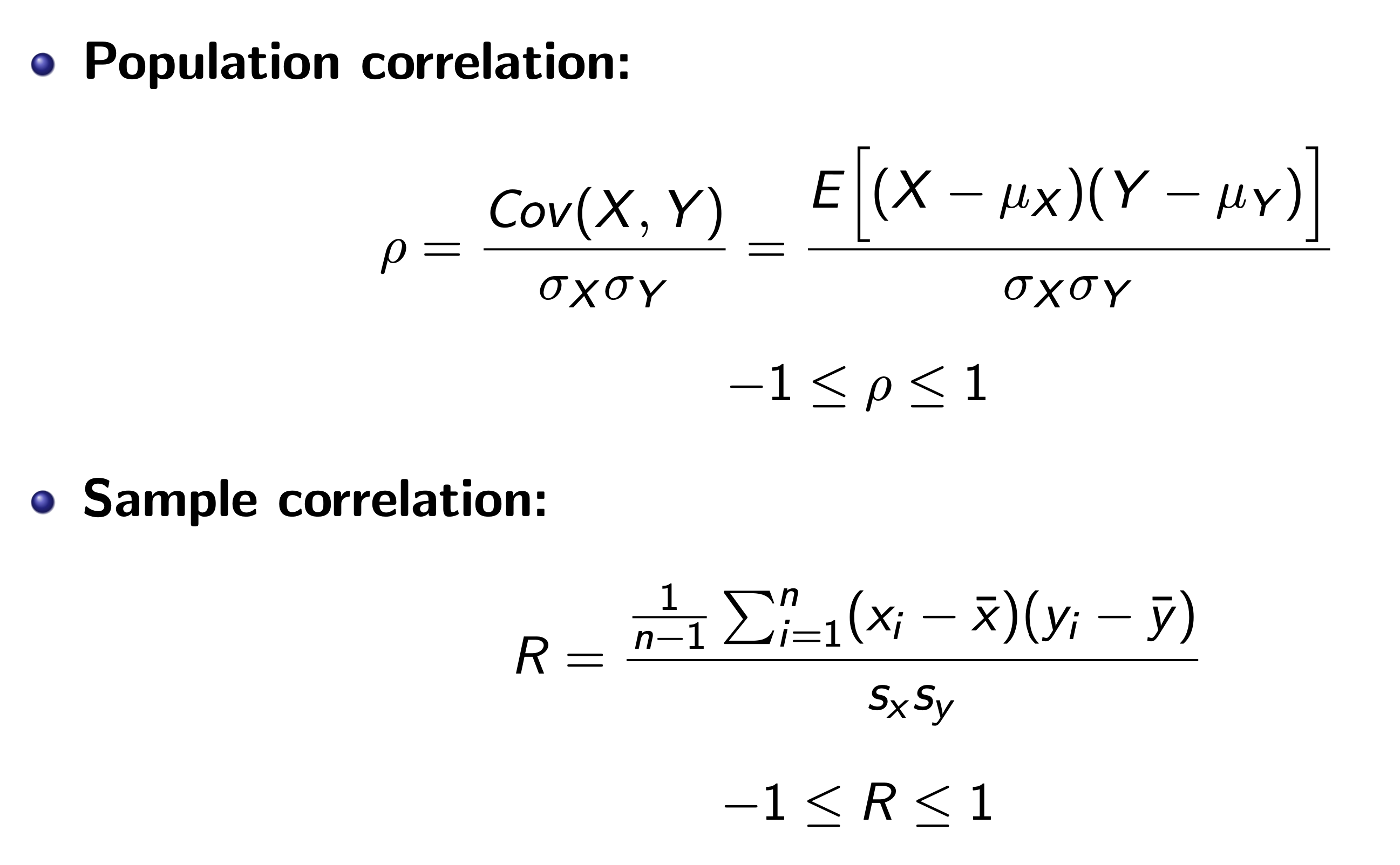
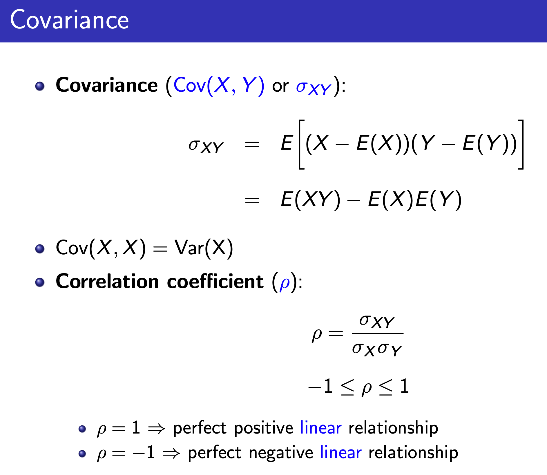
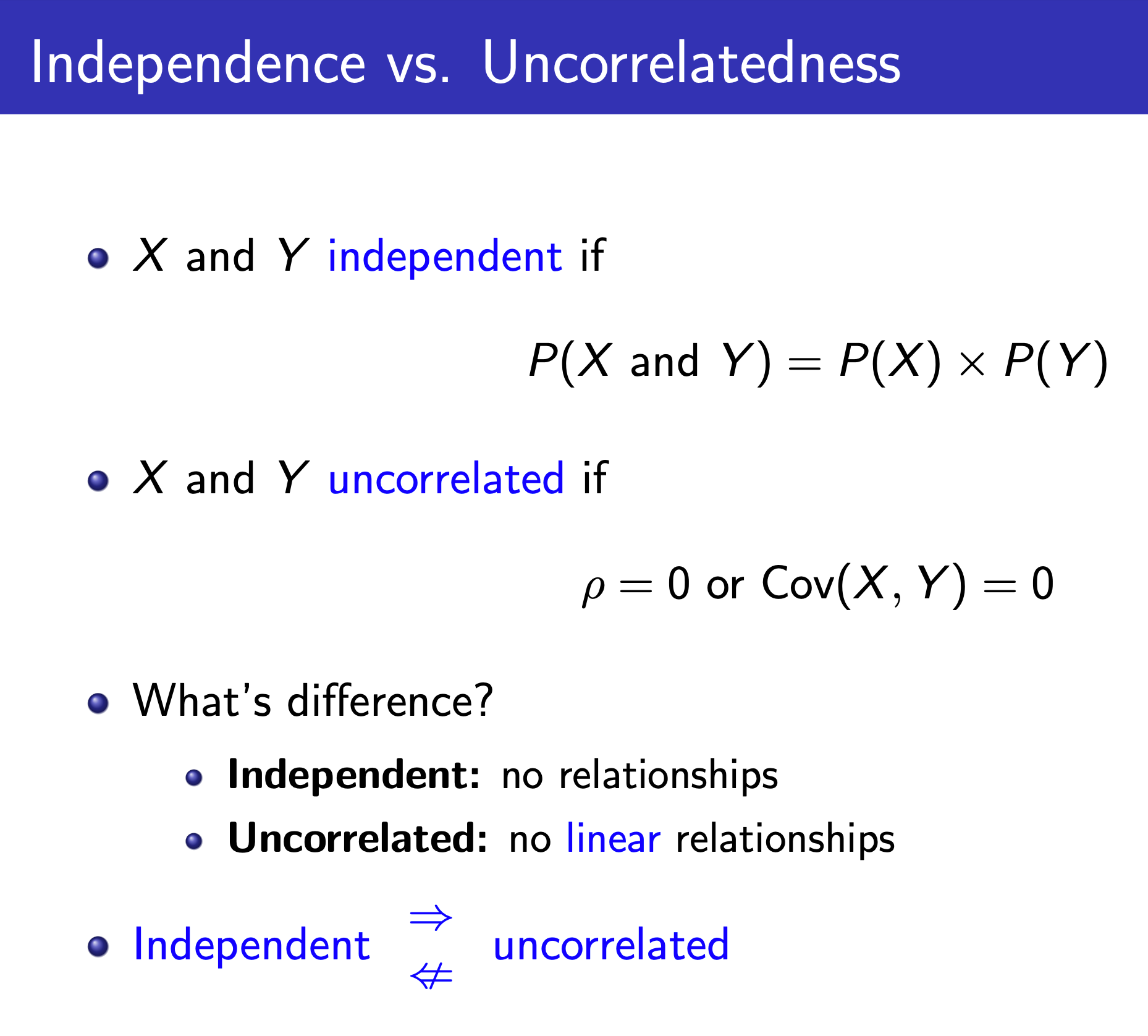
Correlation¶

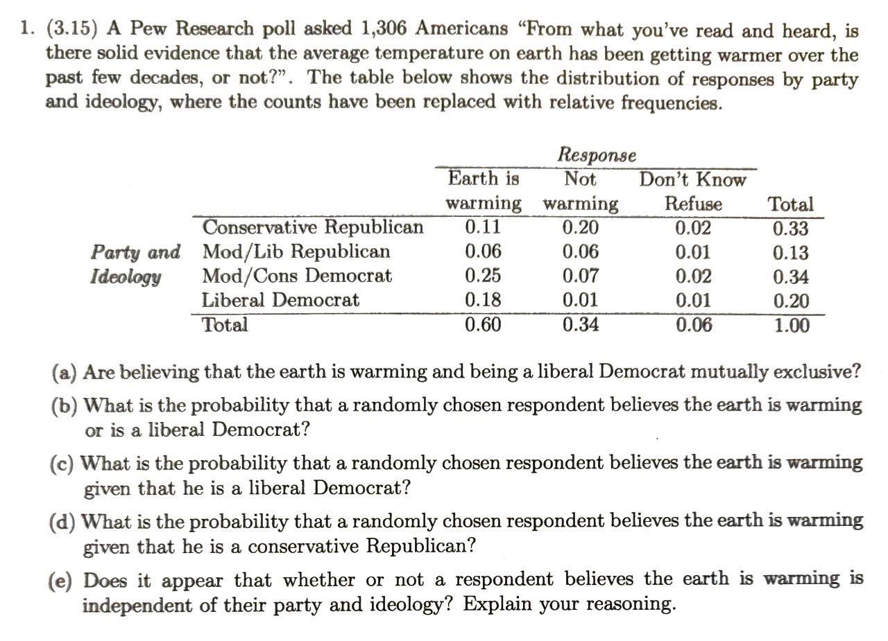
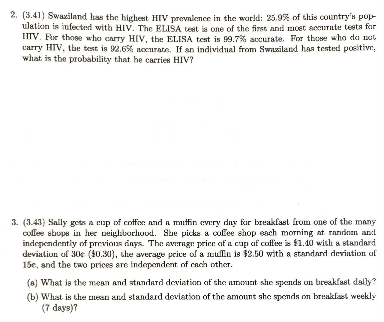
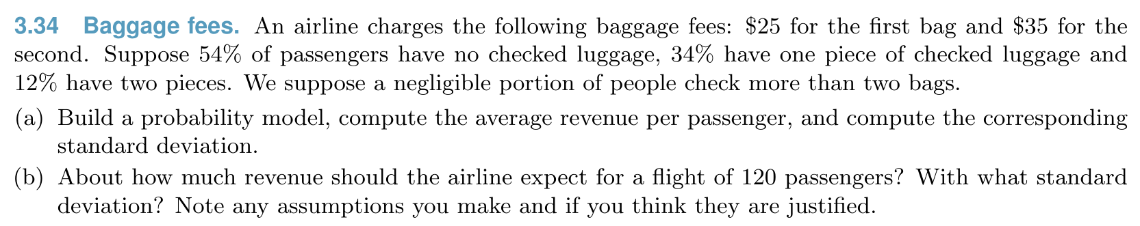
Problems¶

Distribution¶

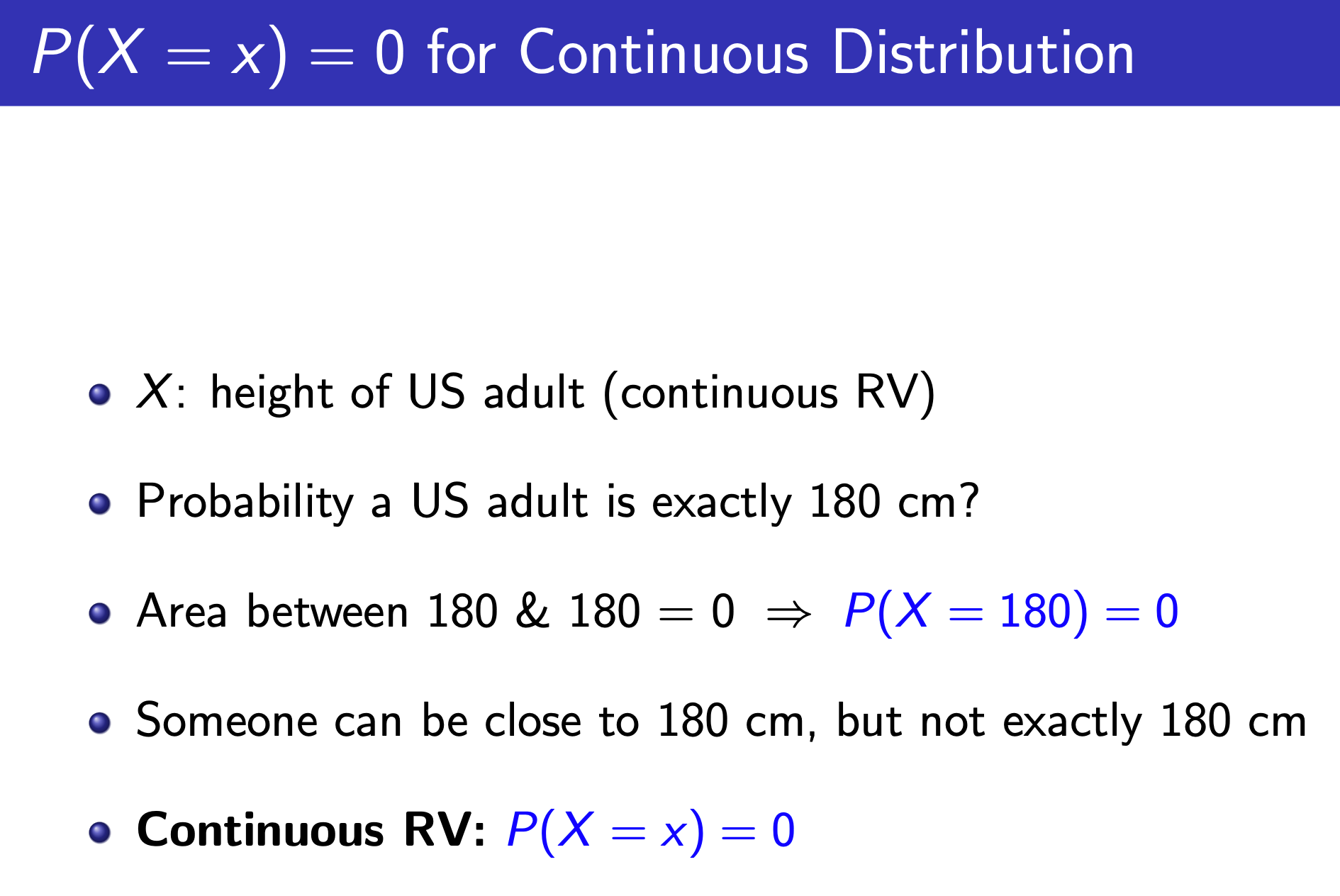
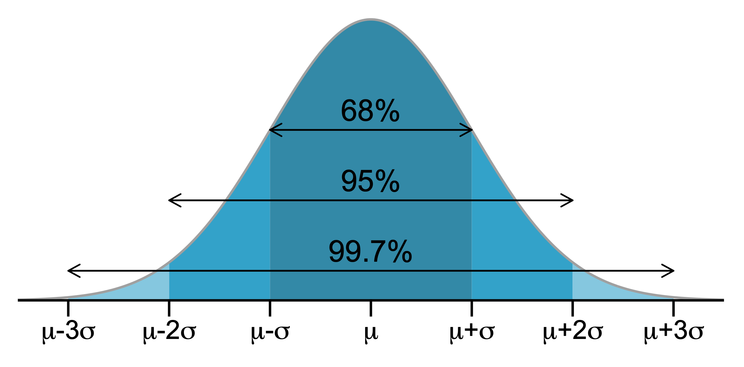
Normal¶

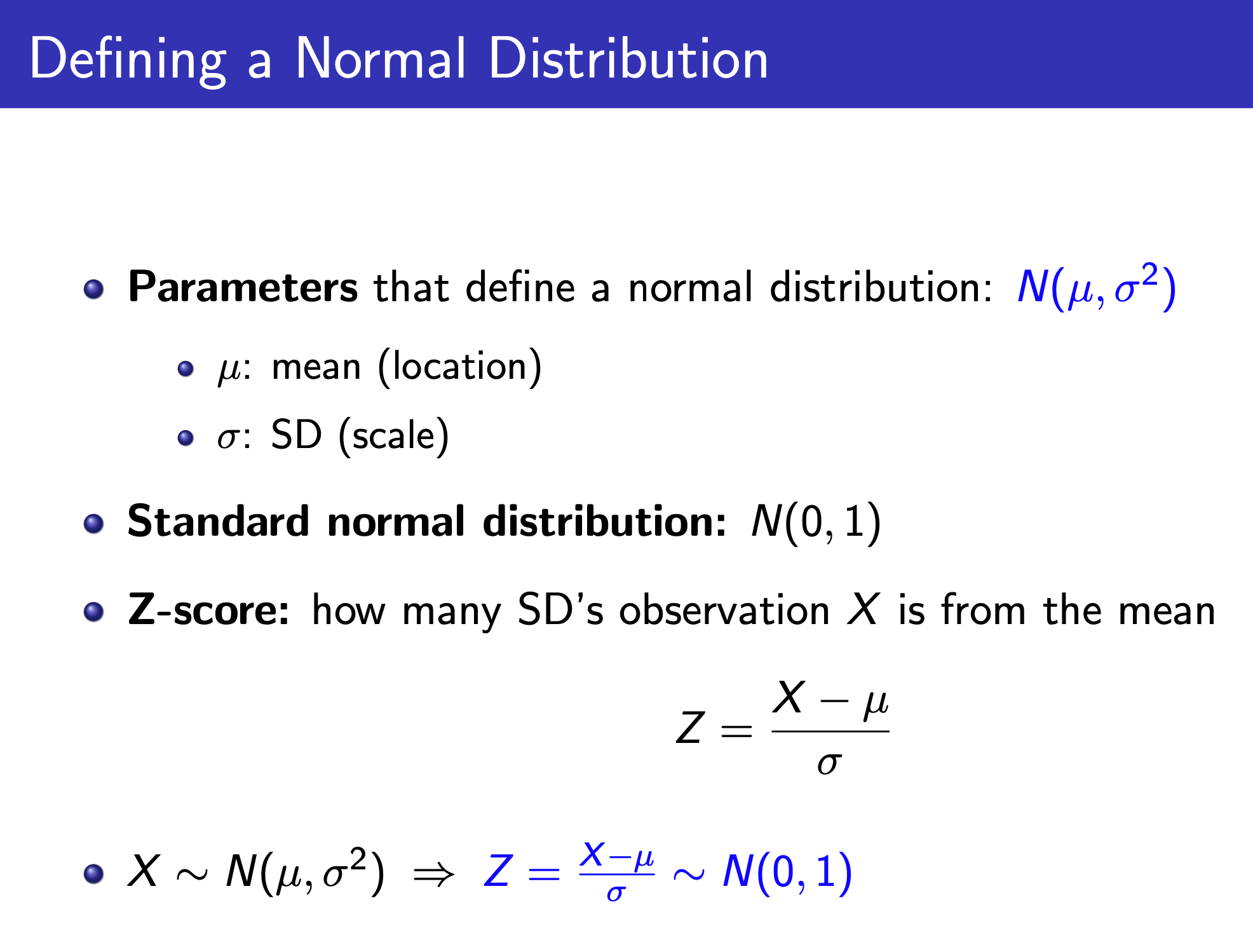
Use z-score to standardize

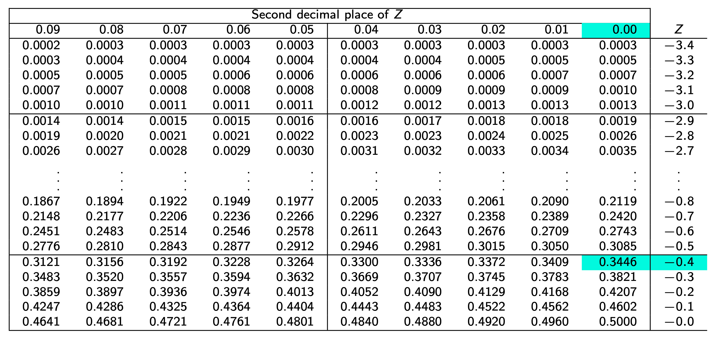
fx-991 es to find probability given z score

https://www.youtube.com/watch?v=bVdQ7OzGvU0

P(z) -> Area less than z value
R(z) -> Area greater than z value
Q(z) -> Area between 0 and z value

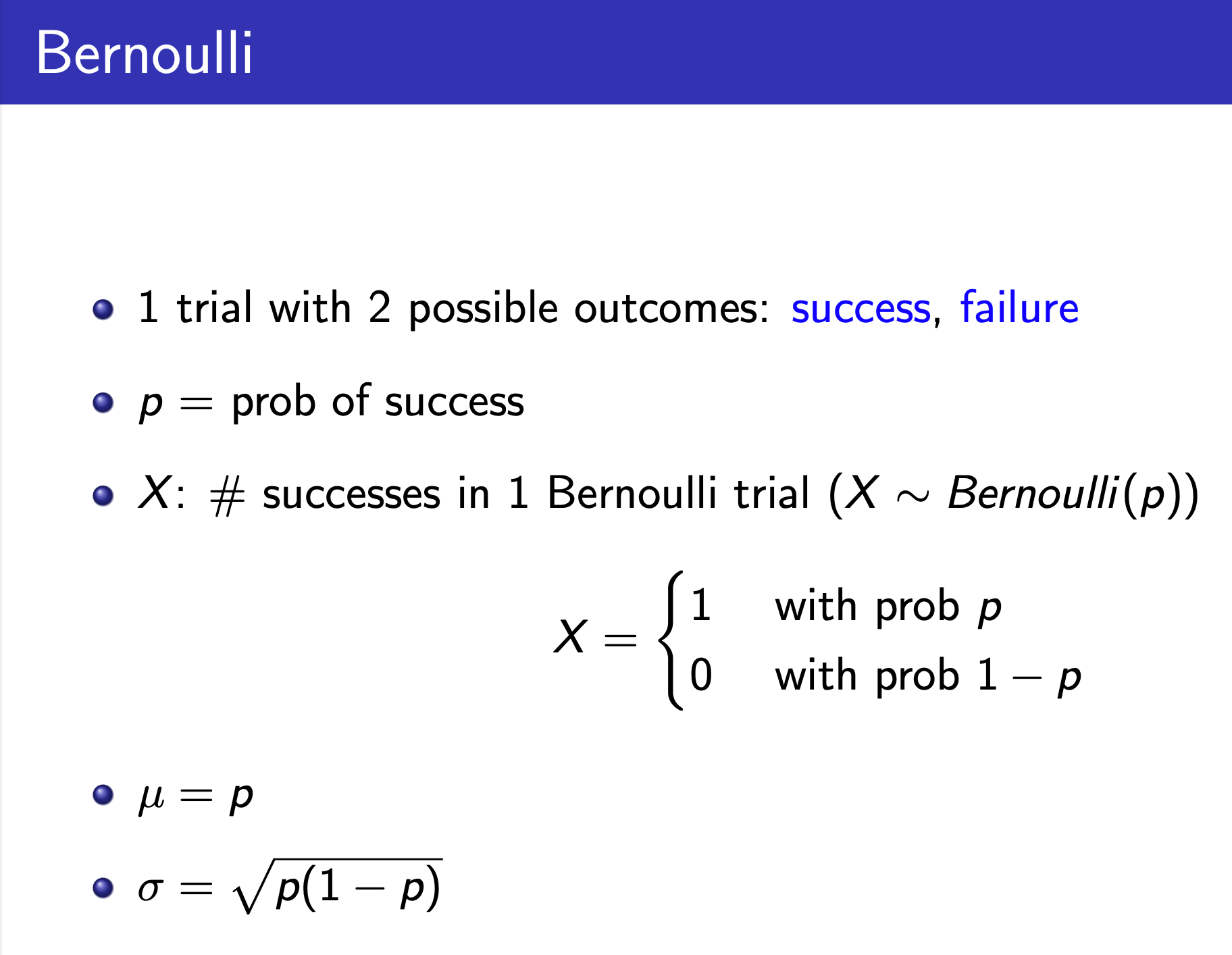
Bernoulli¶

Probability#Bernoulli

\[Var(X)=E(x-\mu)^2=E(x-p)^2=(1-p)^2p+(0-p)^2(1-p)=p(1-p)\]

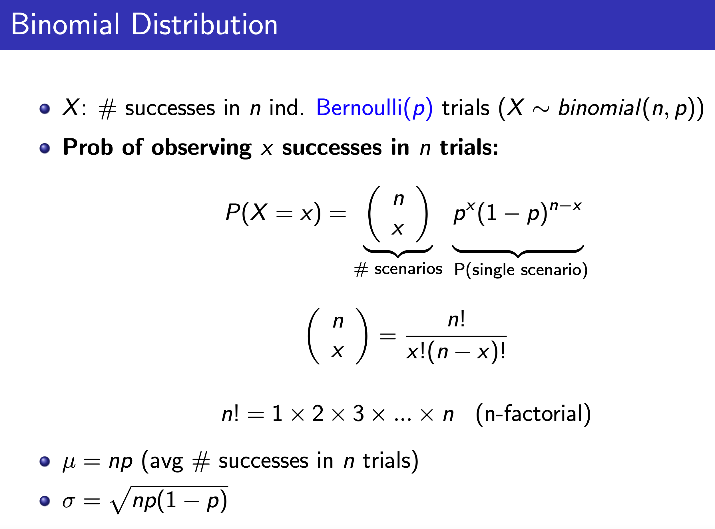
Binomial¶

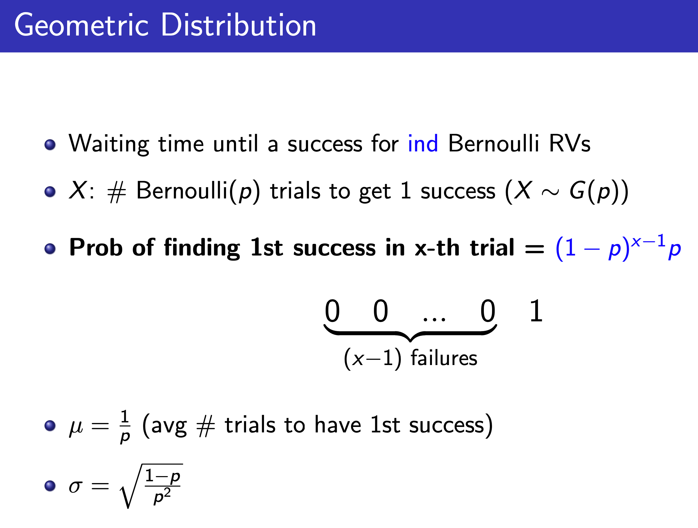
Geometric¶

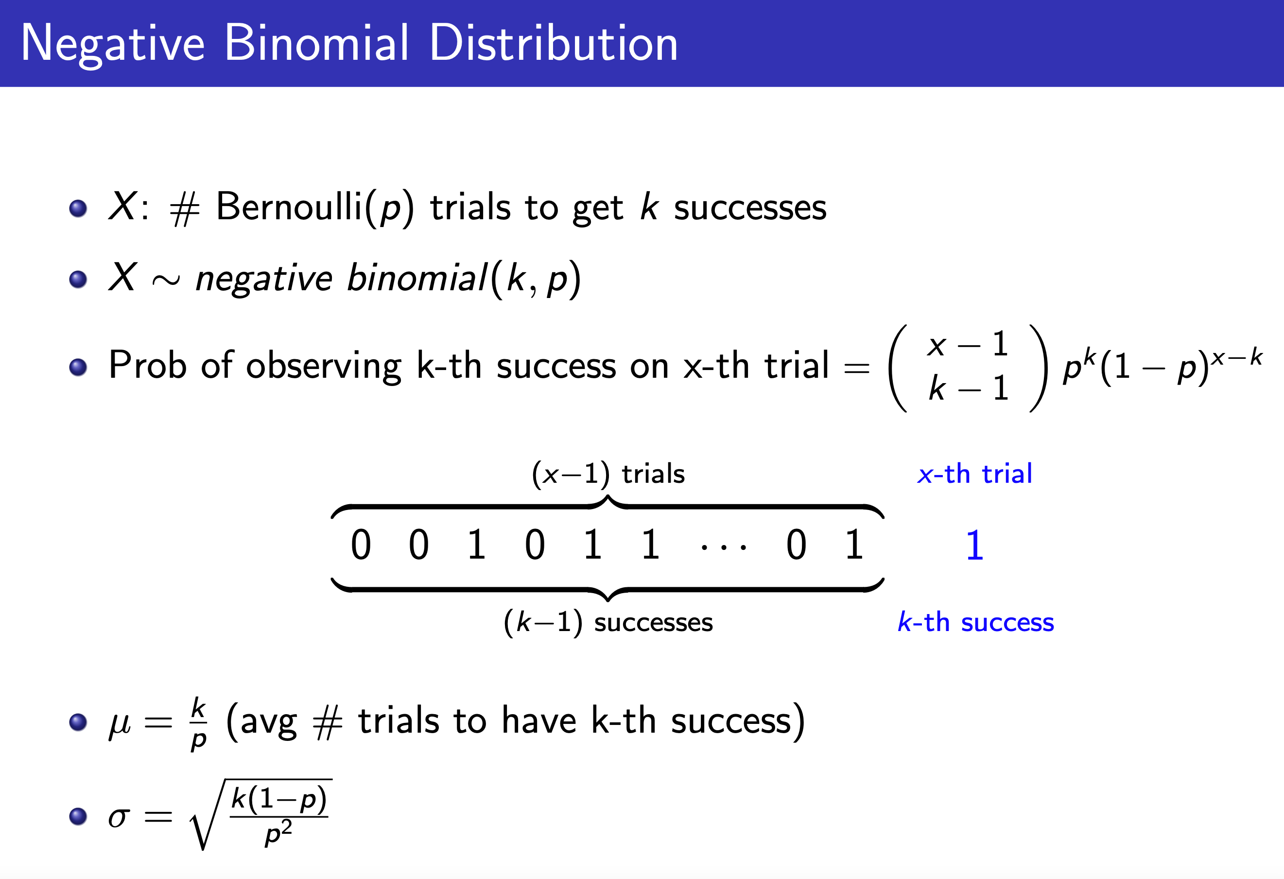
Negative Binomial / Pascal¶

i.e. Pascal

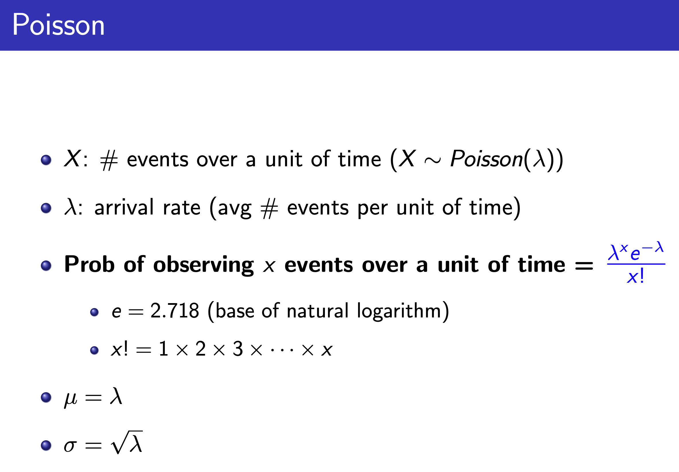
Poisson¶

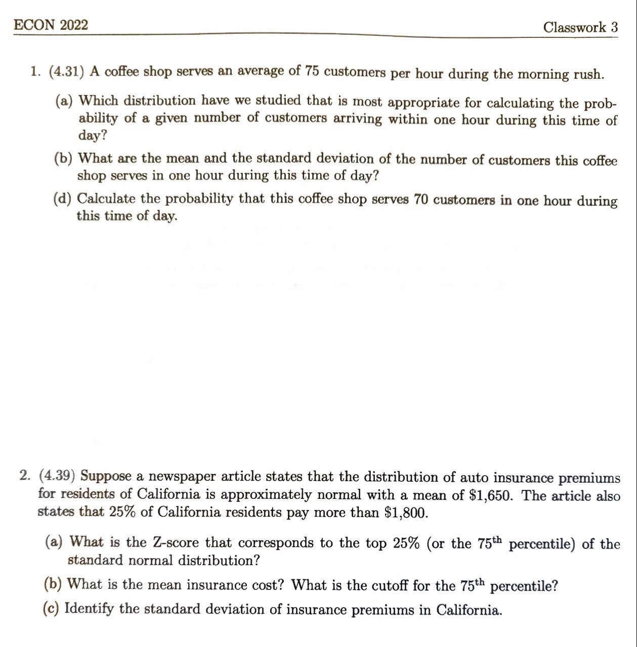
Problems¶

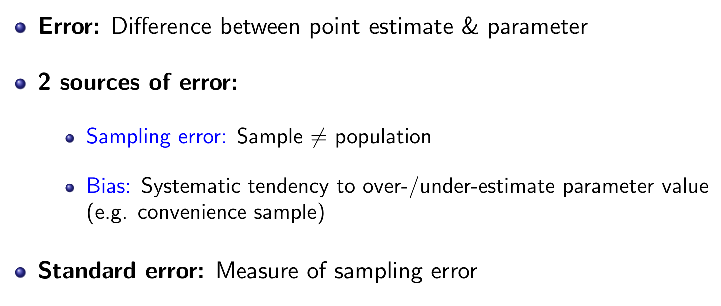
Foundation of Inference¶

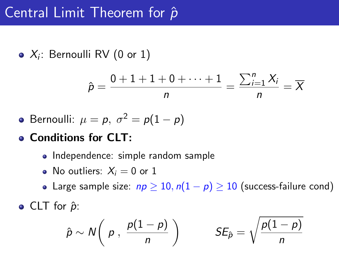
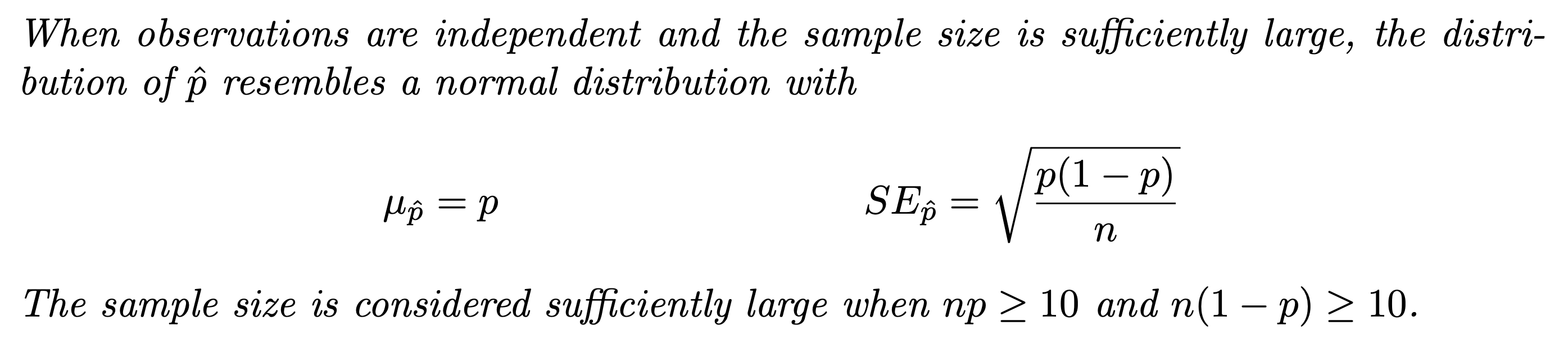
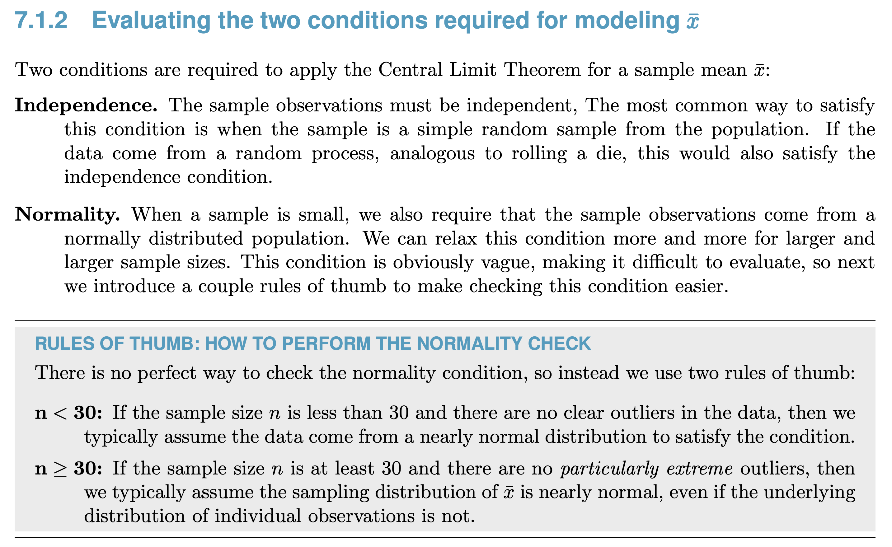
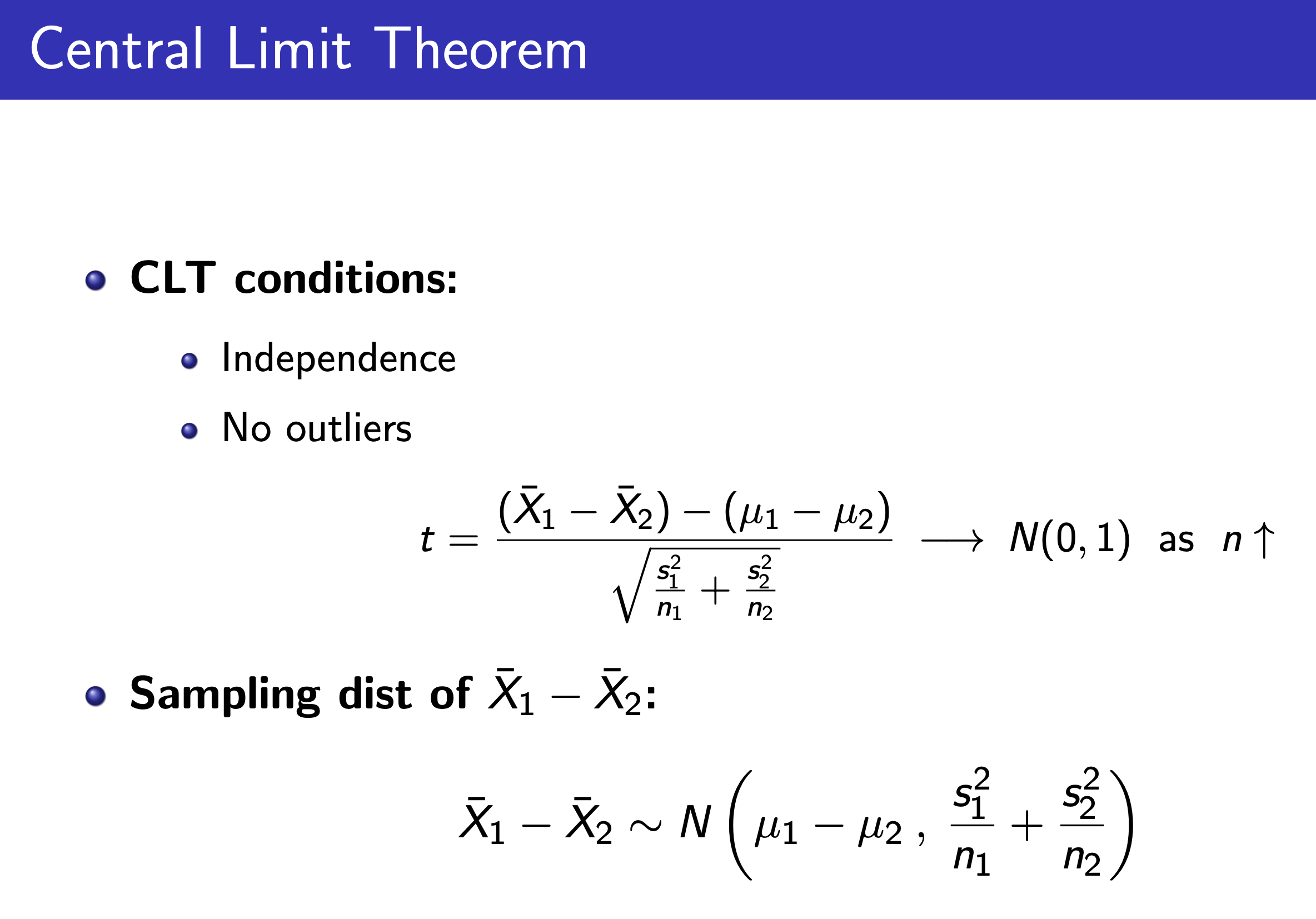
Central Limit Theorem¶

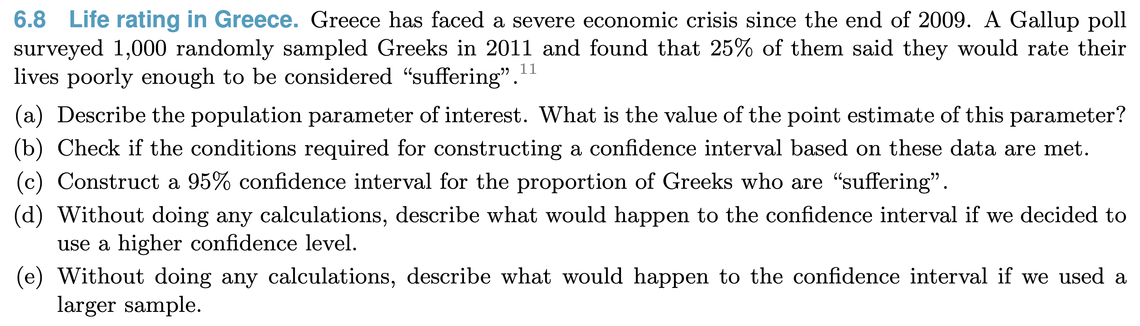
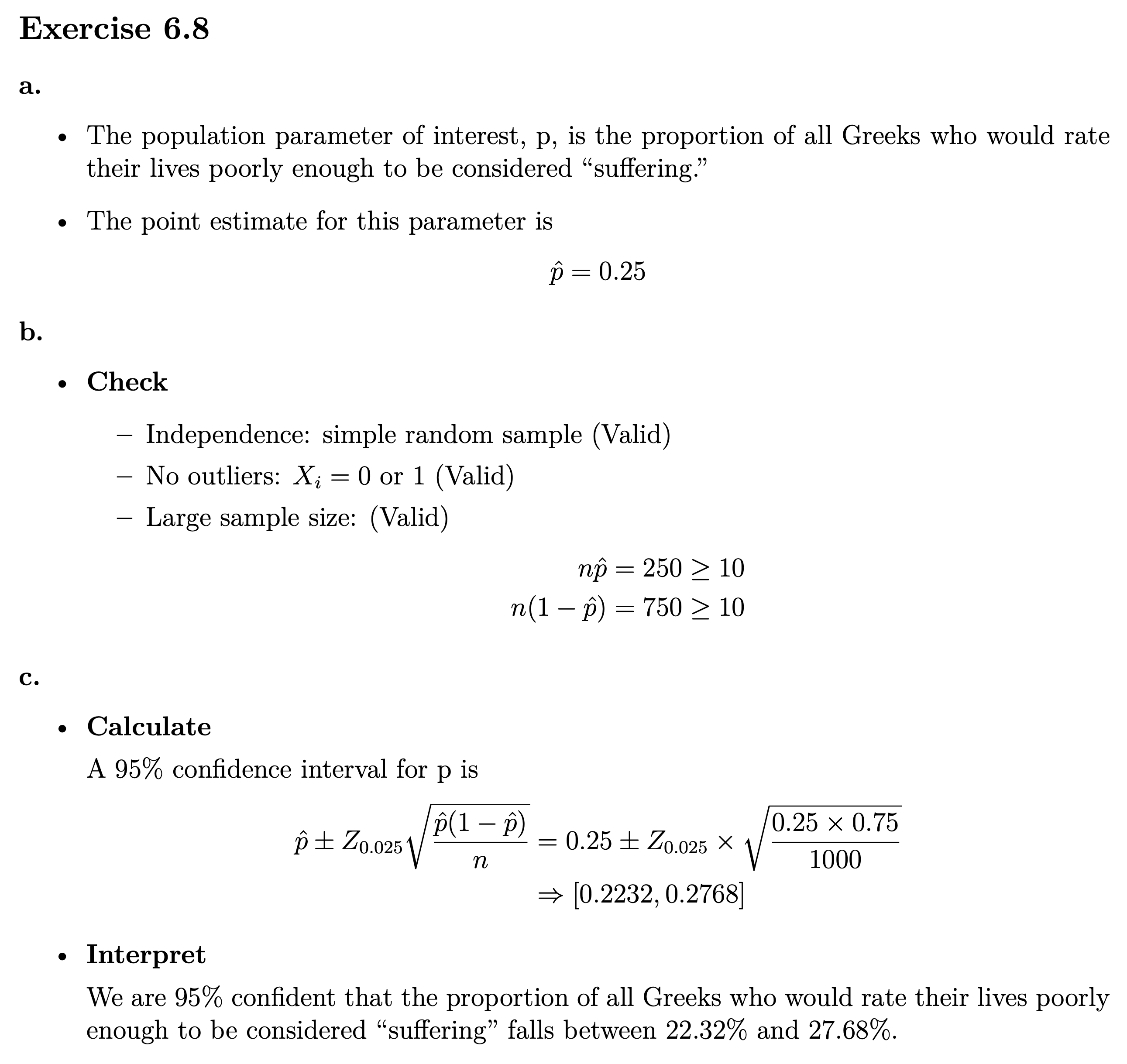
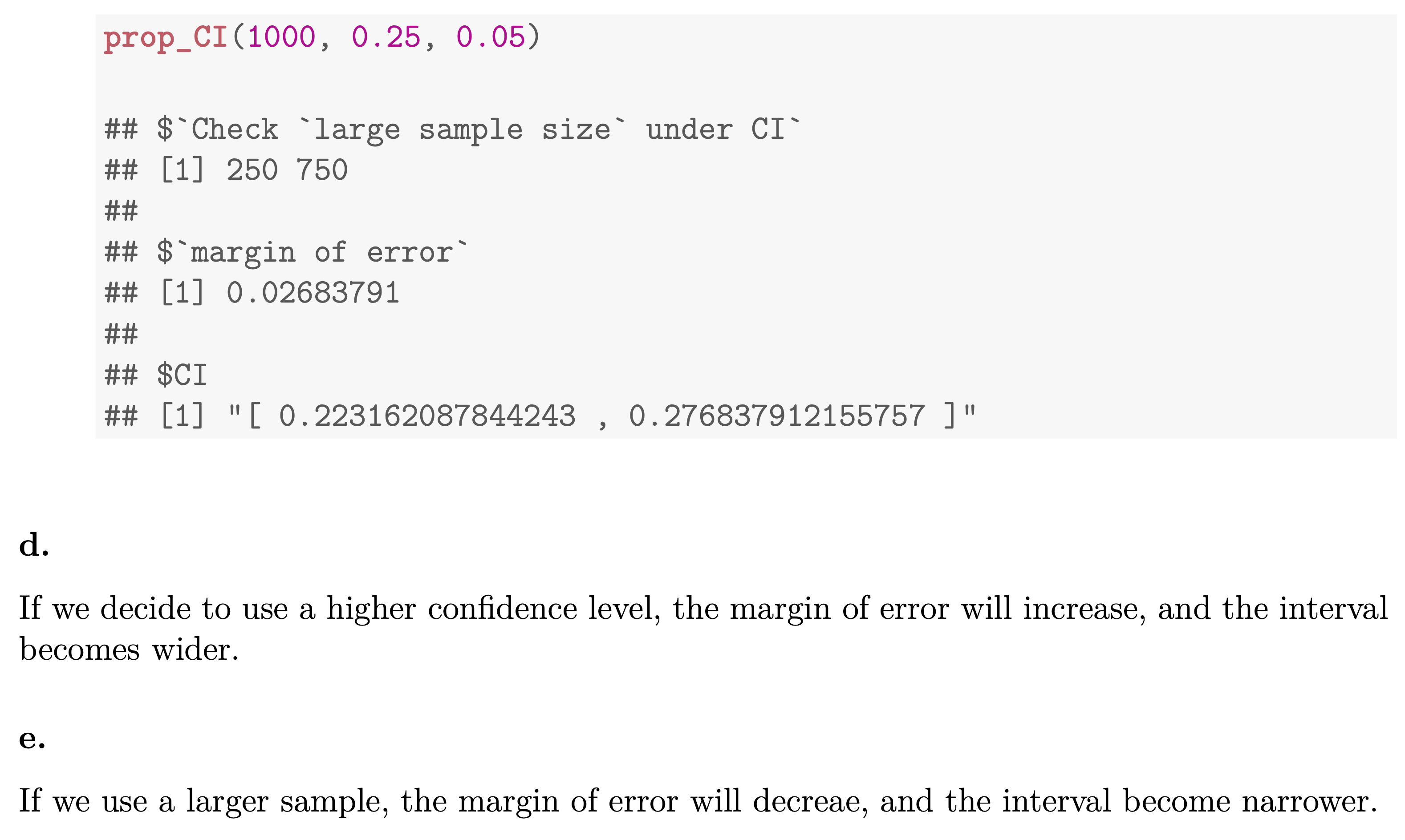
Confidence Interval¶

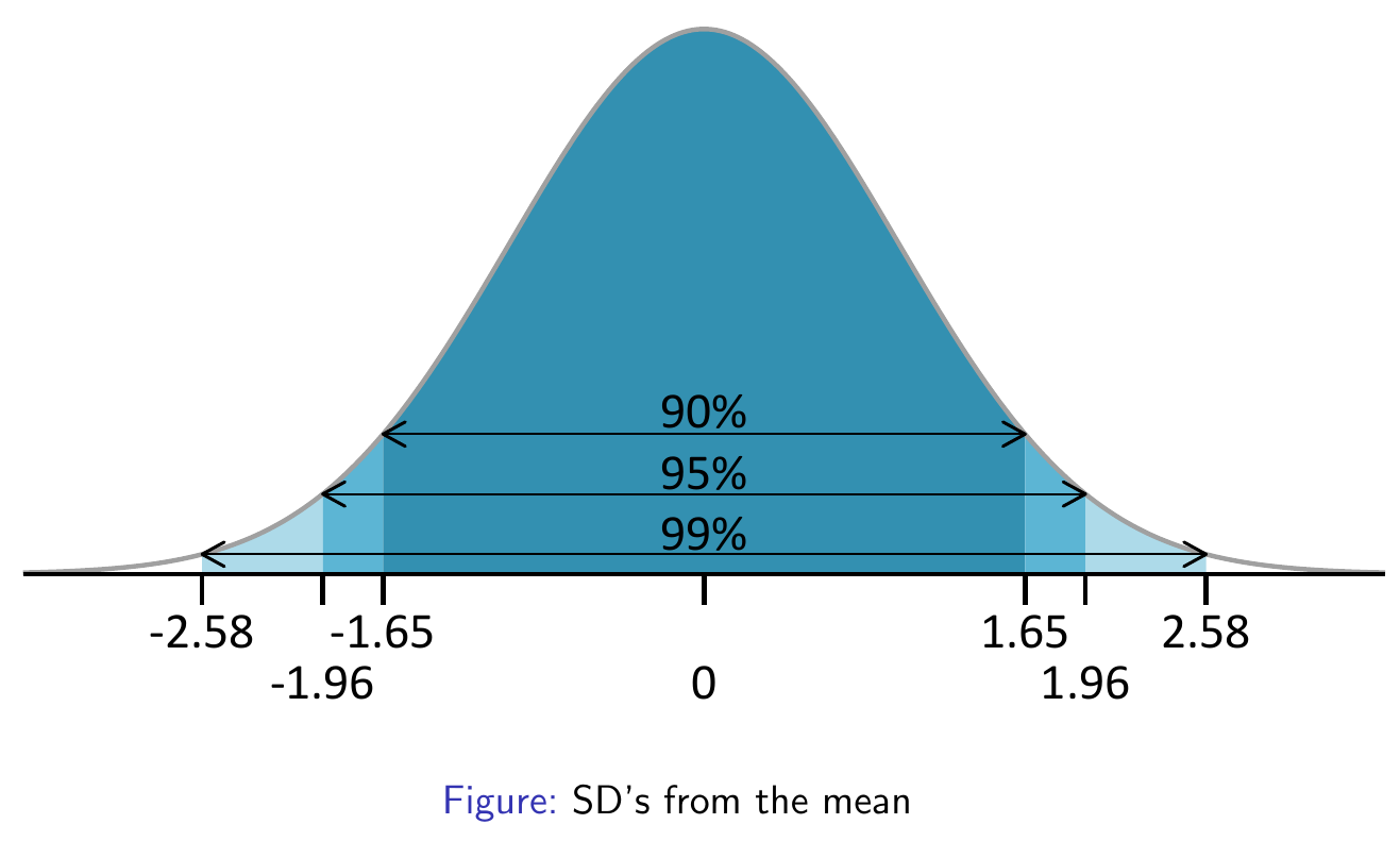
Confidence Interval
99%: 2.5758 = 2.576 = 2.58
95%: 1.9600 = 1.960 = 1.96
90%: 1.6449 = 1.645 = 1.65

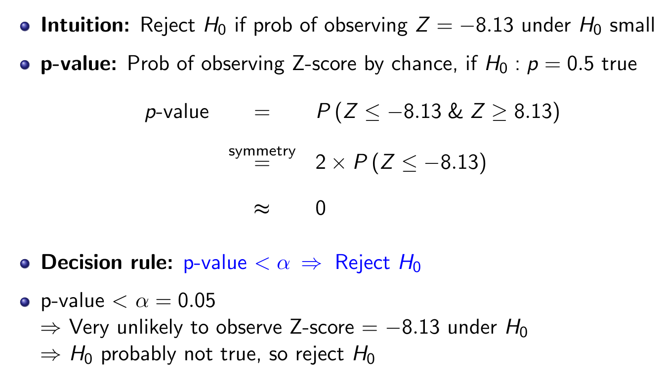
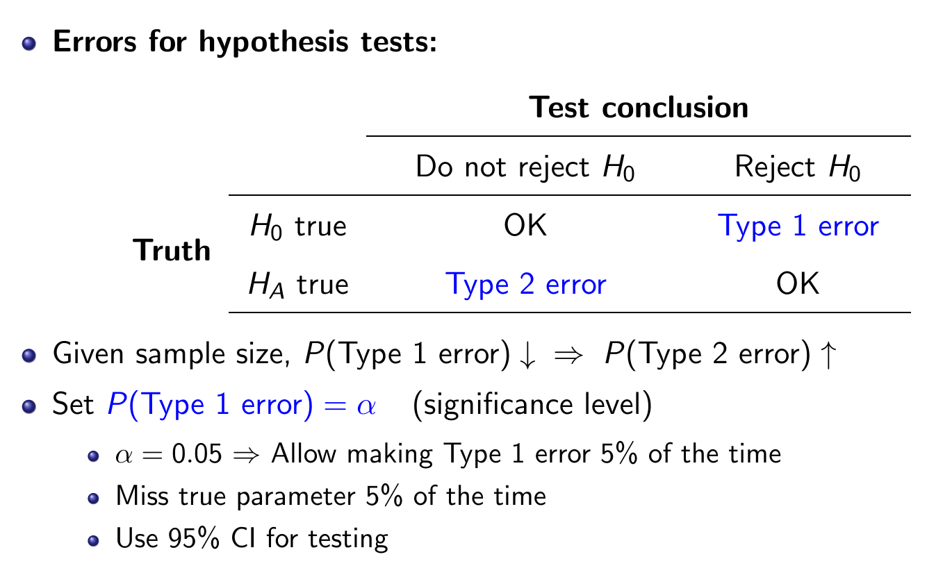
Hypothesis Testing¶

\(\alpha\) means the critical p value i.e. significance level

Type 1 Error = False Positive
- assuming null -> negative, reject null -> positive
Type 2 Error = False Negative

Remember to use the p stated in \(H_0\) to calculate SE and do hypothesis testing!

e.g.

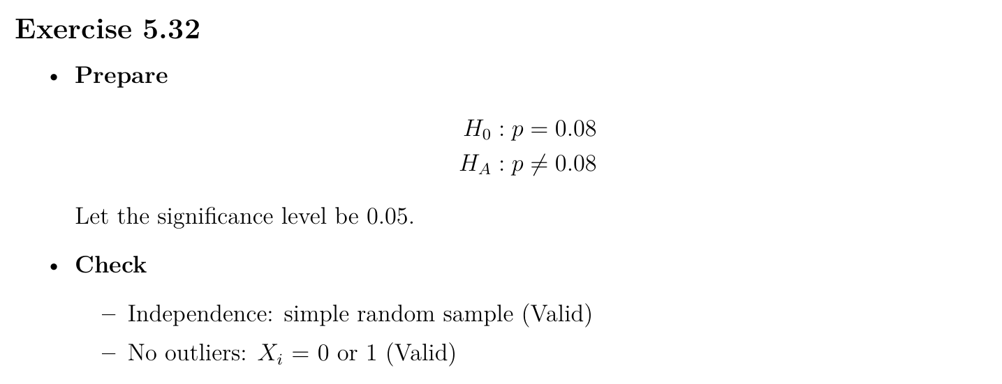
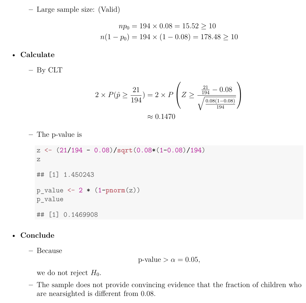
There is no statistically significant evidence that the fraction of children who are nearsighted is different from 0.08 at the 5% level

Inference for Categorical Data¶

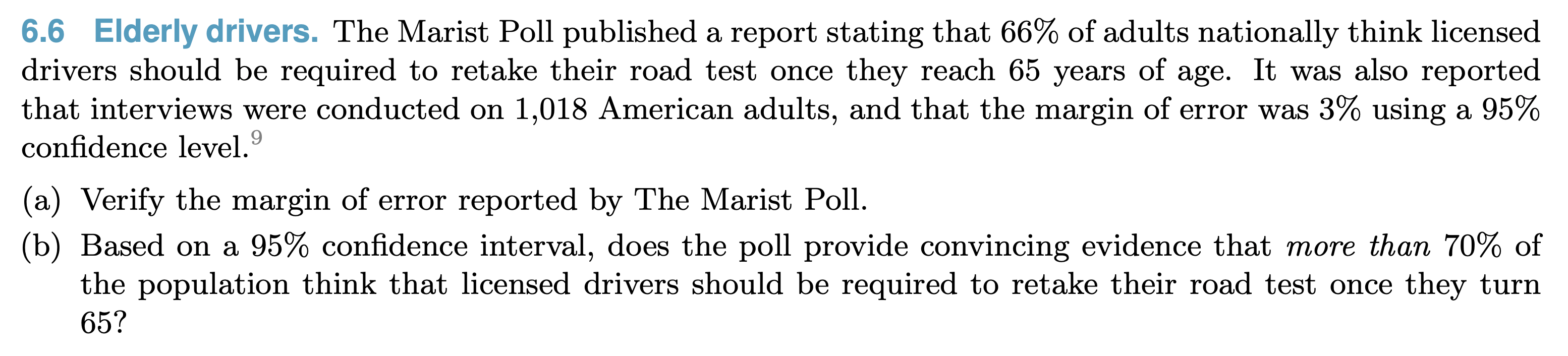
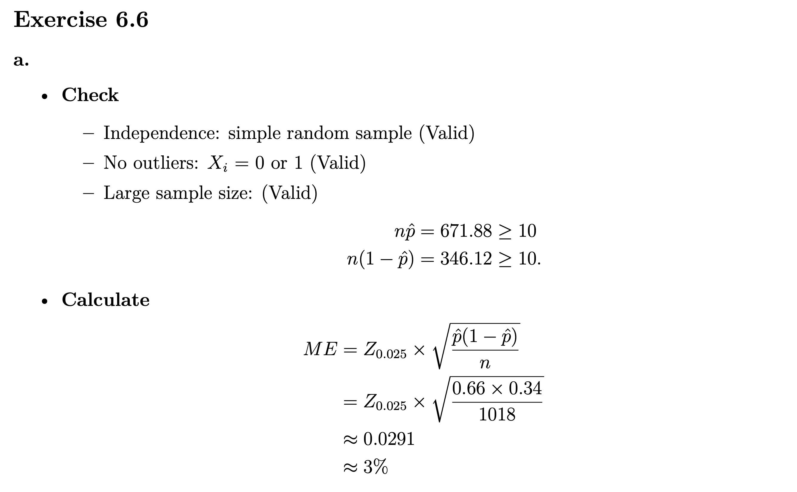
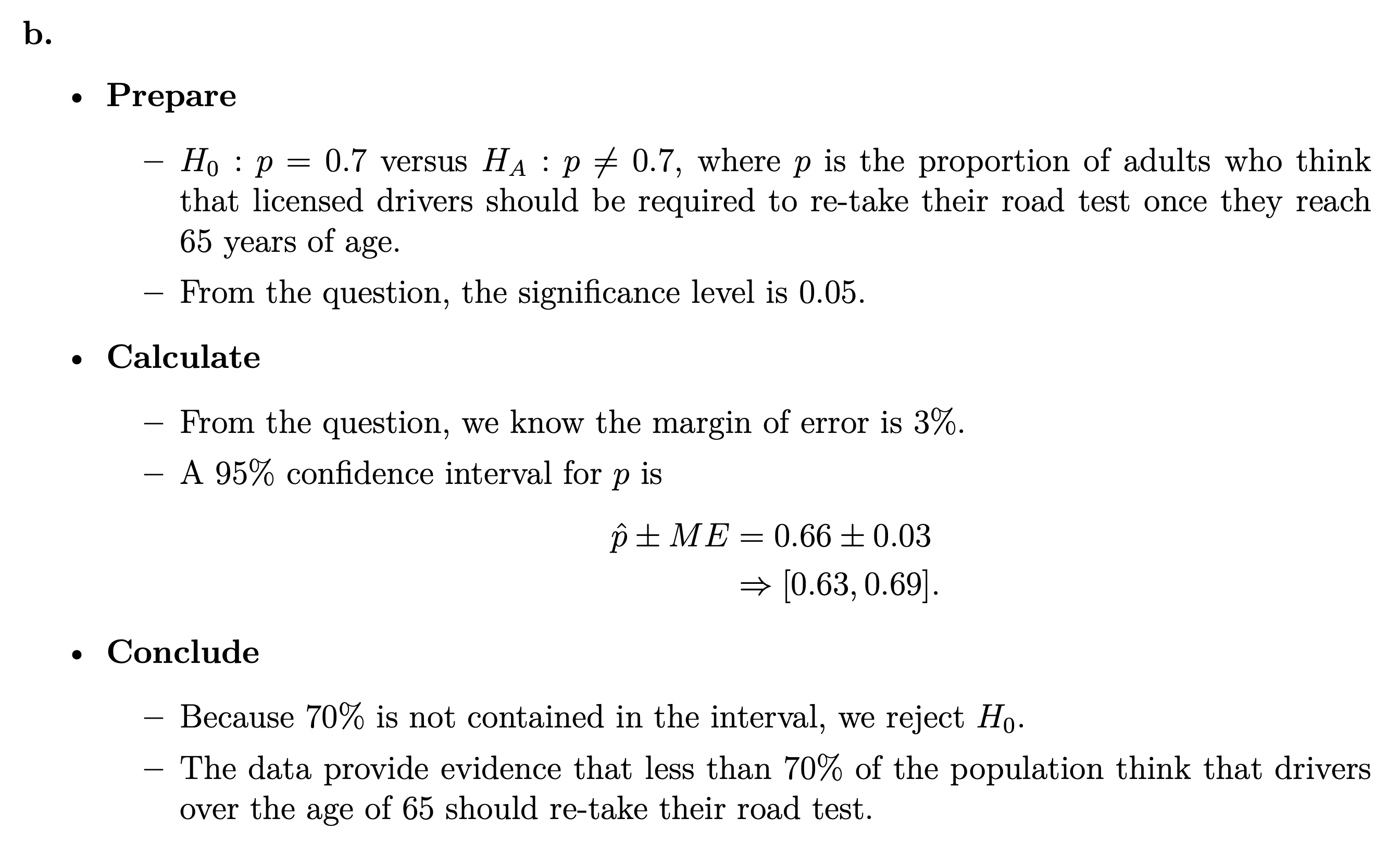
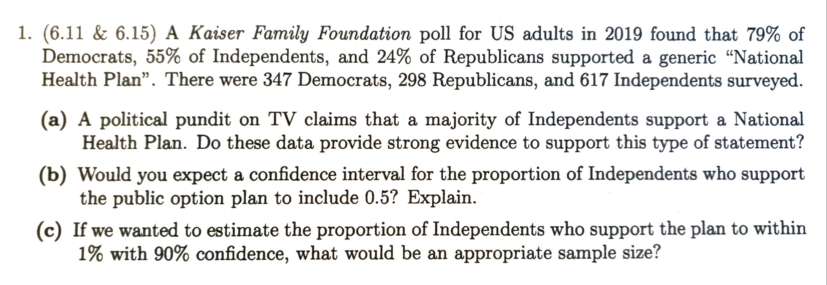
Hypothesis Testing for 1 Porportion¶

Problems¶

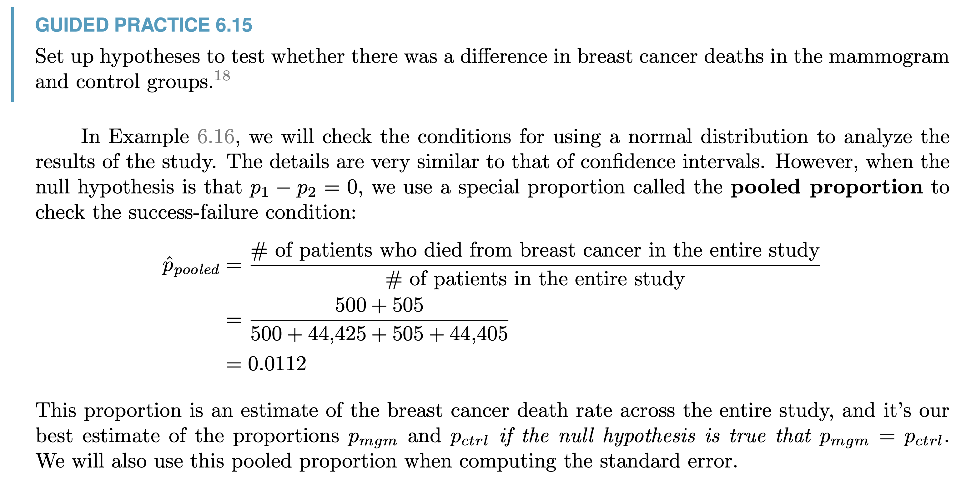
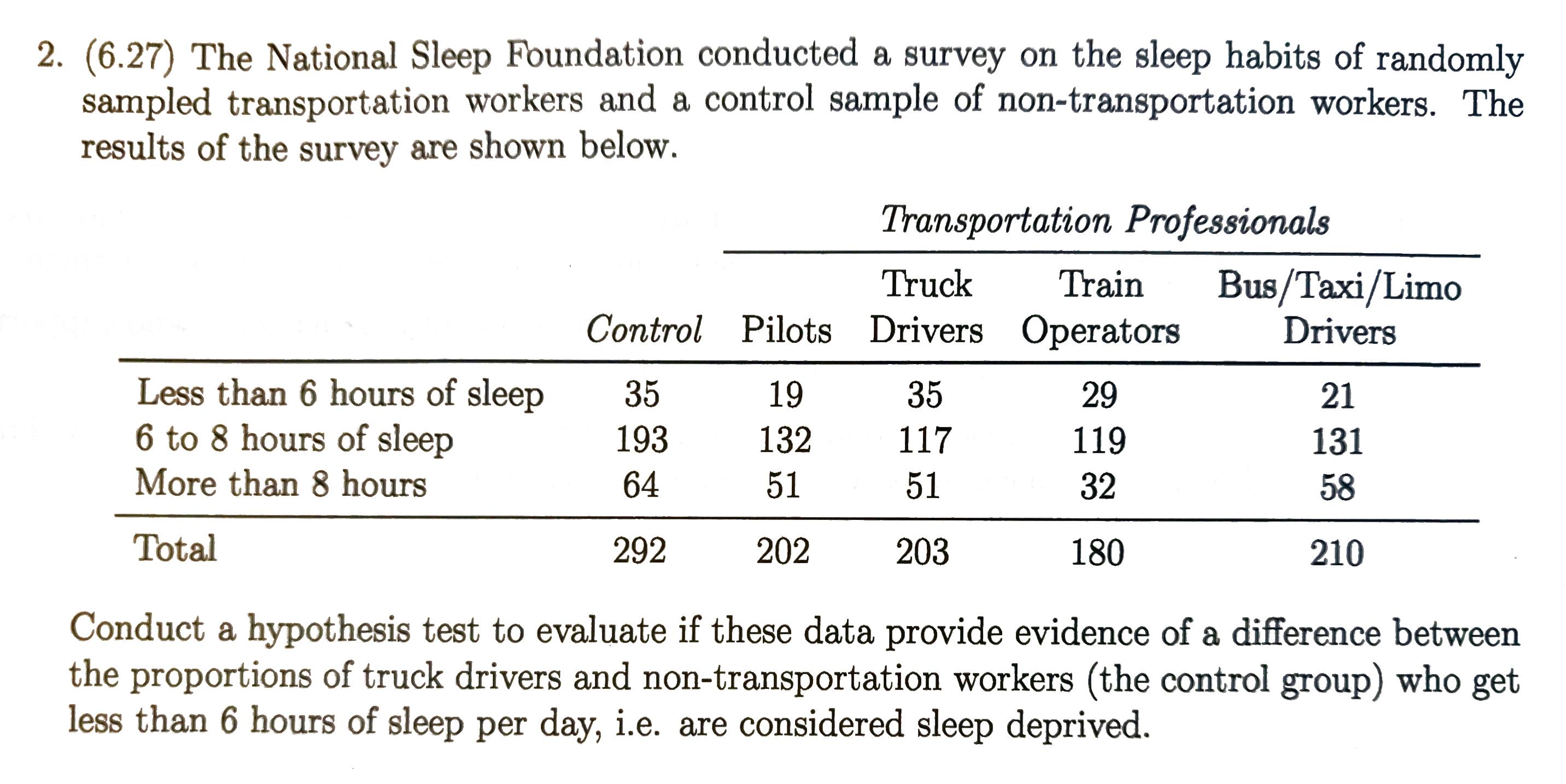
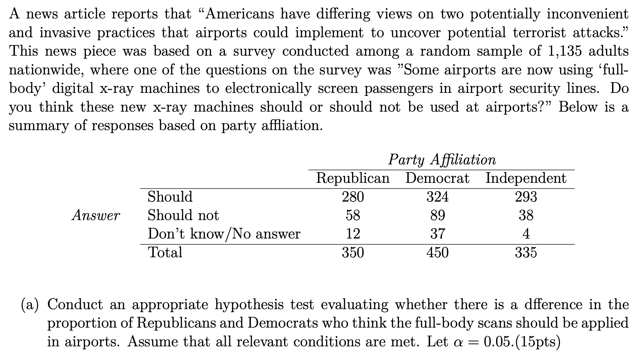
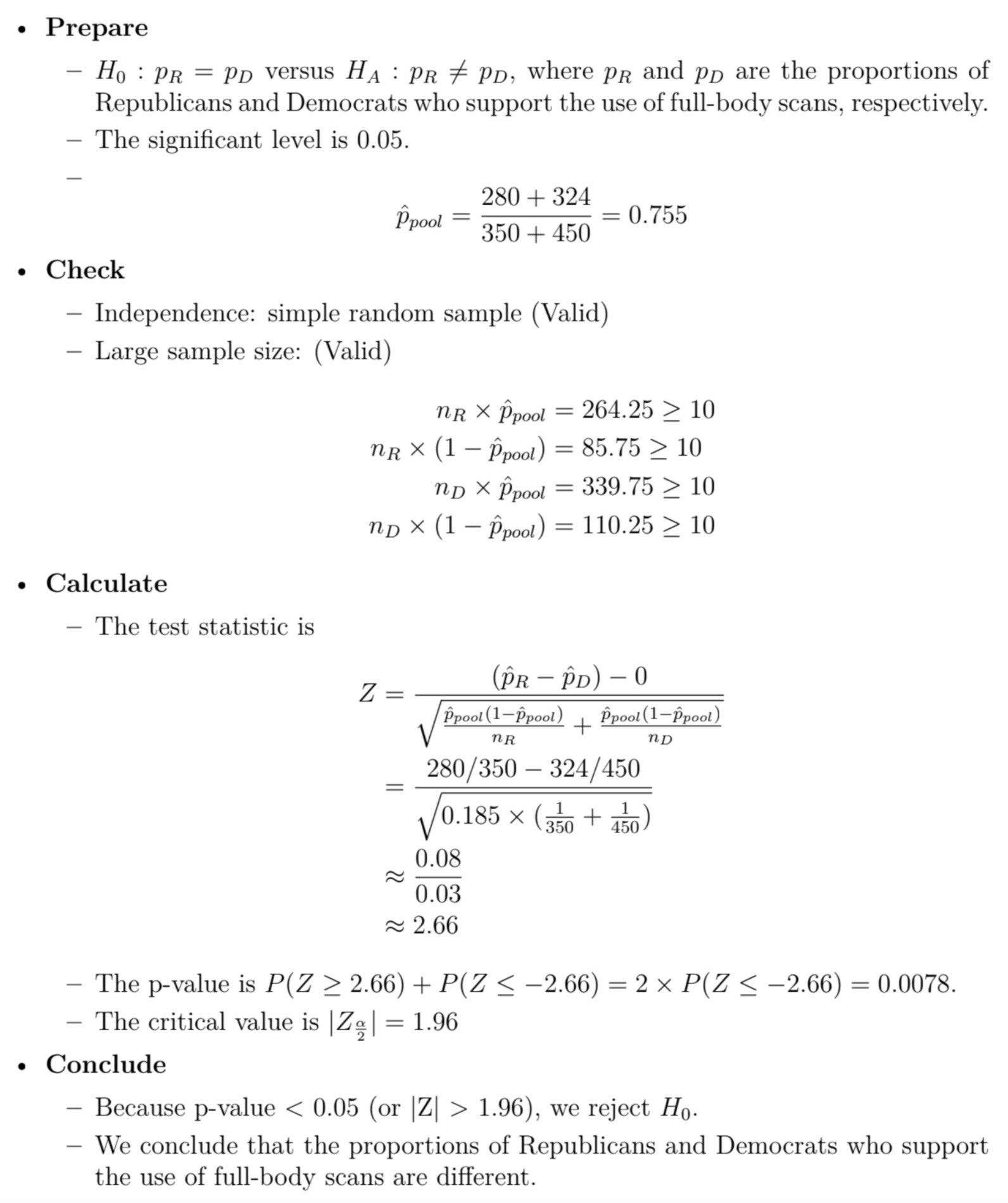
Hypothesis Testing for 2 Porportion¶

SE of the difference between 2 porportions

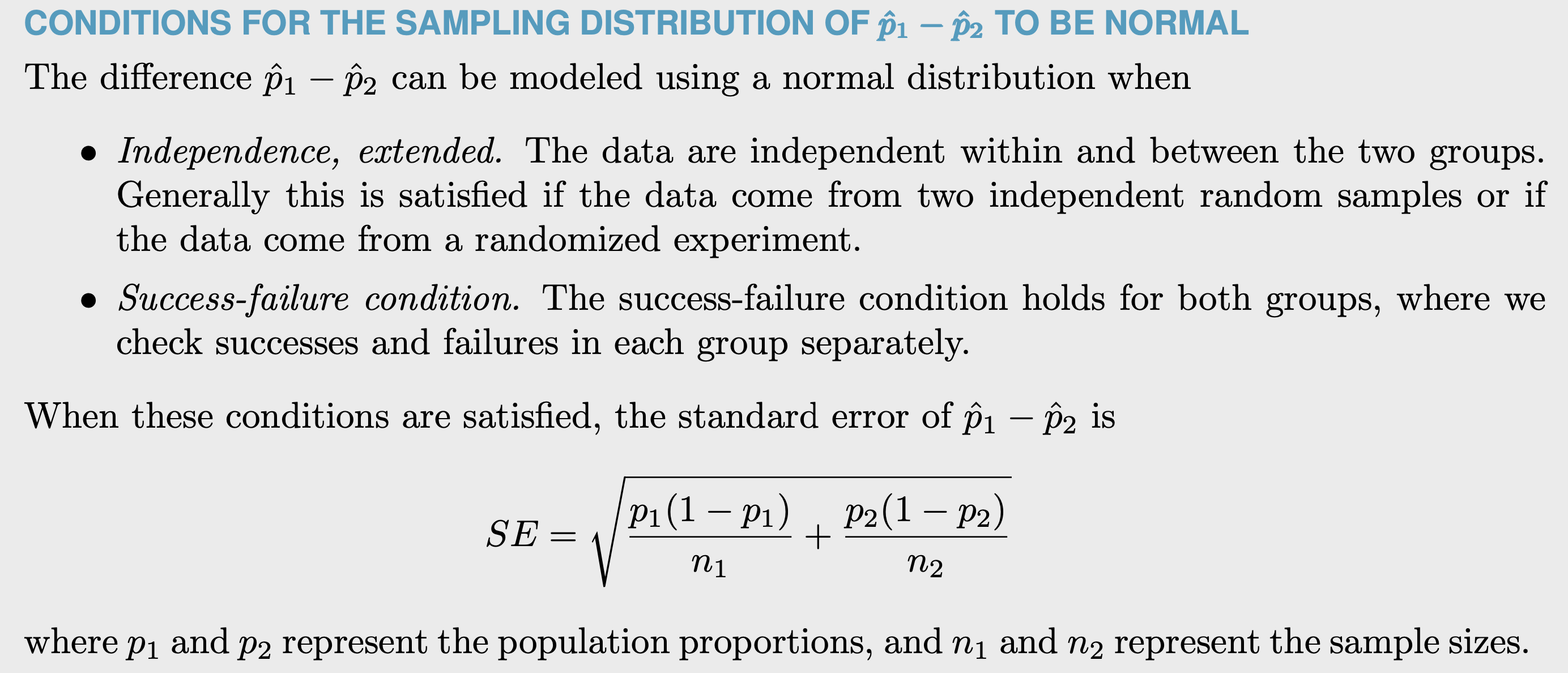
e.g.

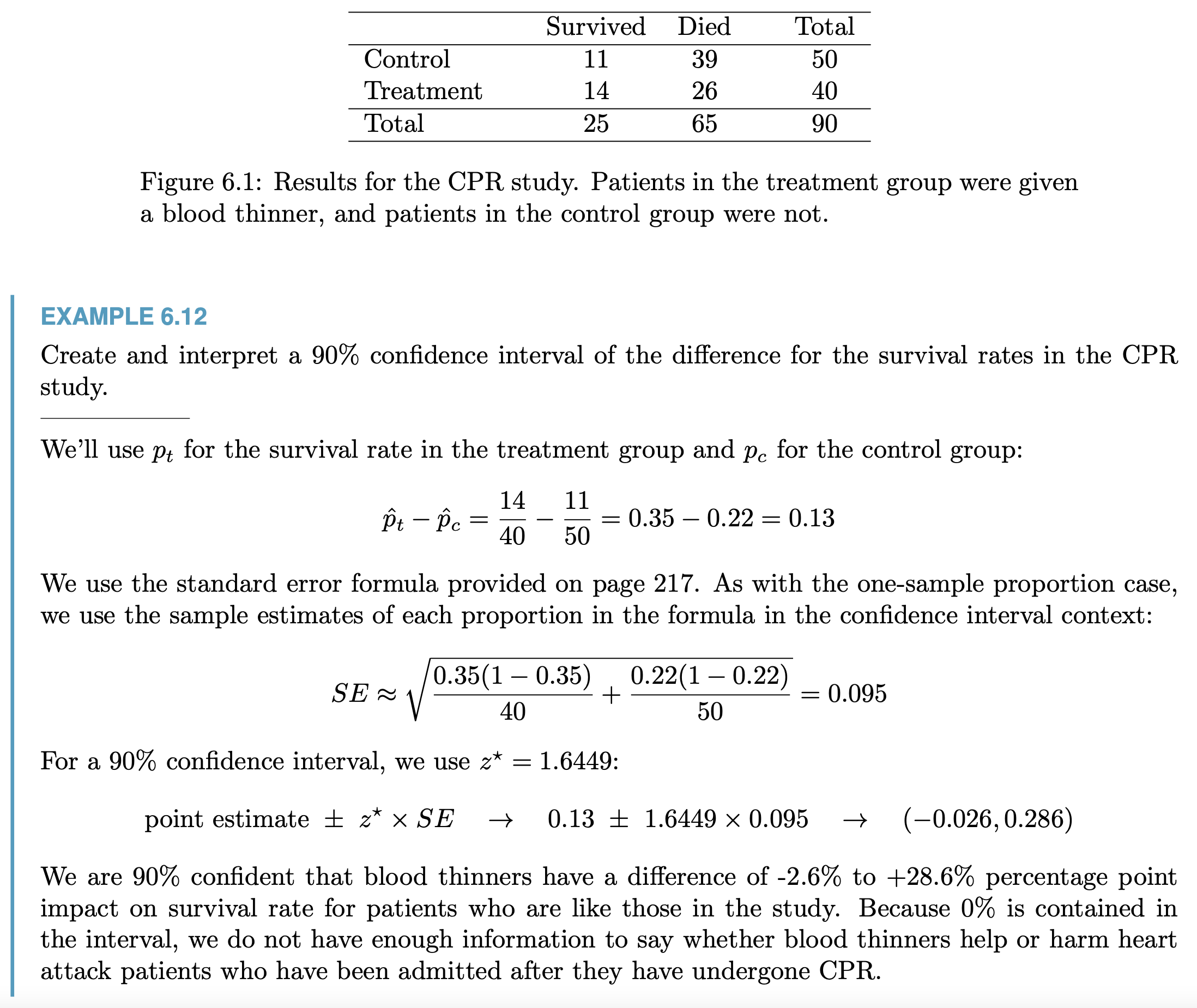
Use p = overall p of the 2 porportions to calculate SE when \(H_0\) is that 2 porportions has the same mean

Problems¶

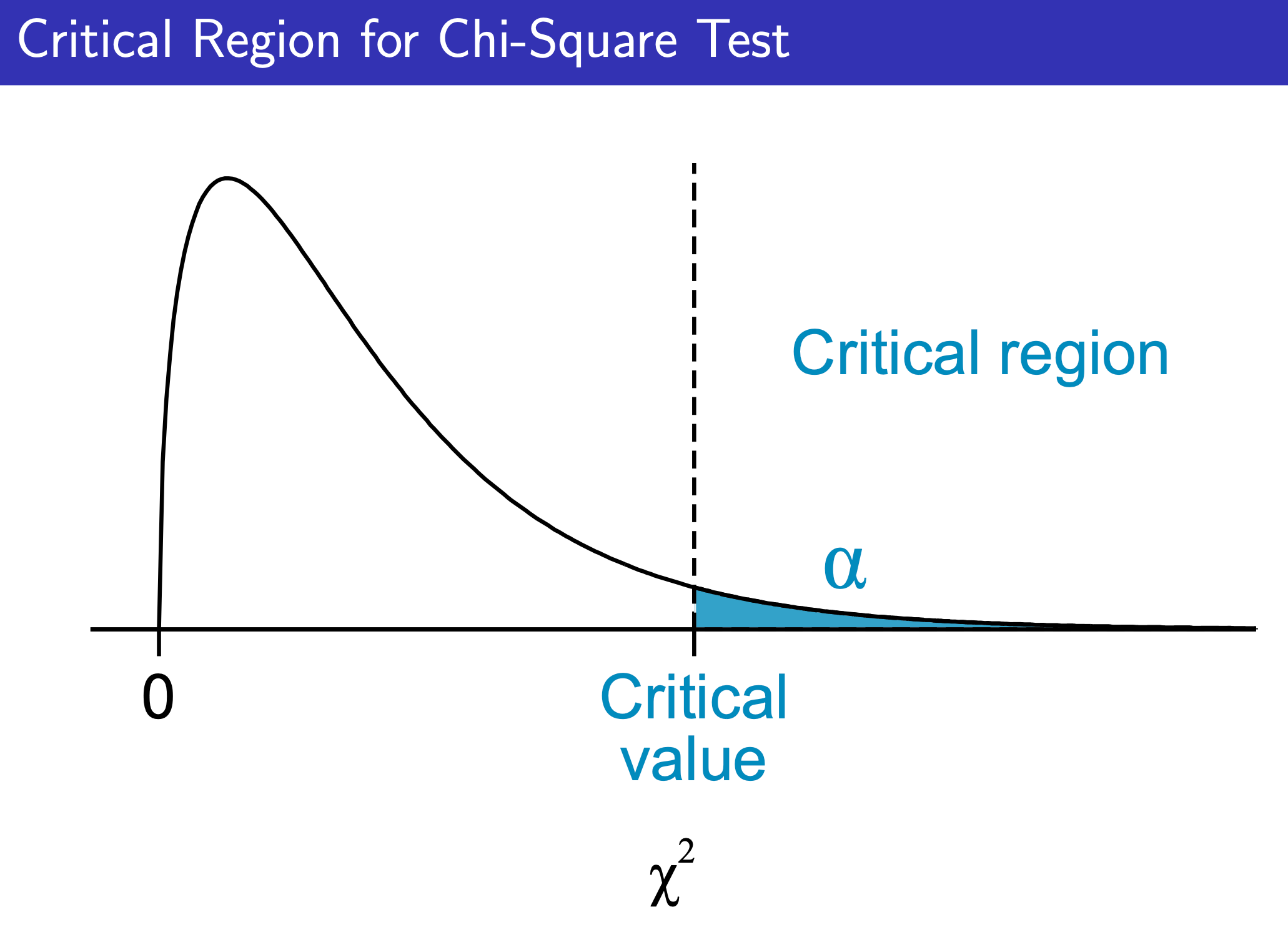
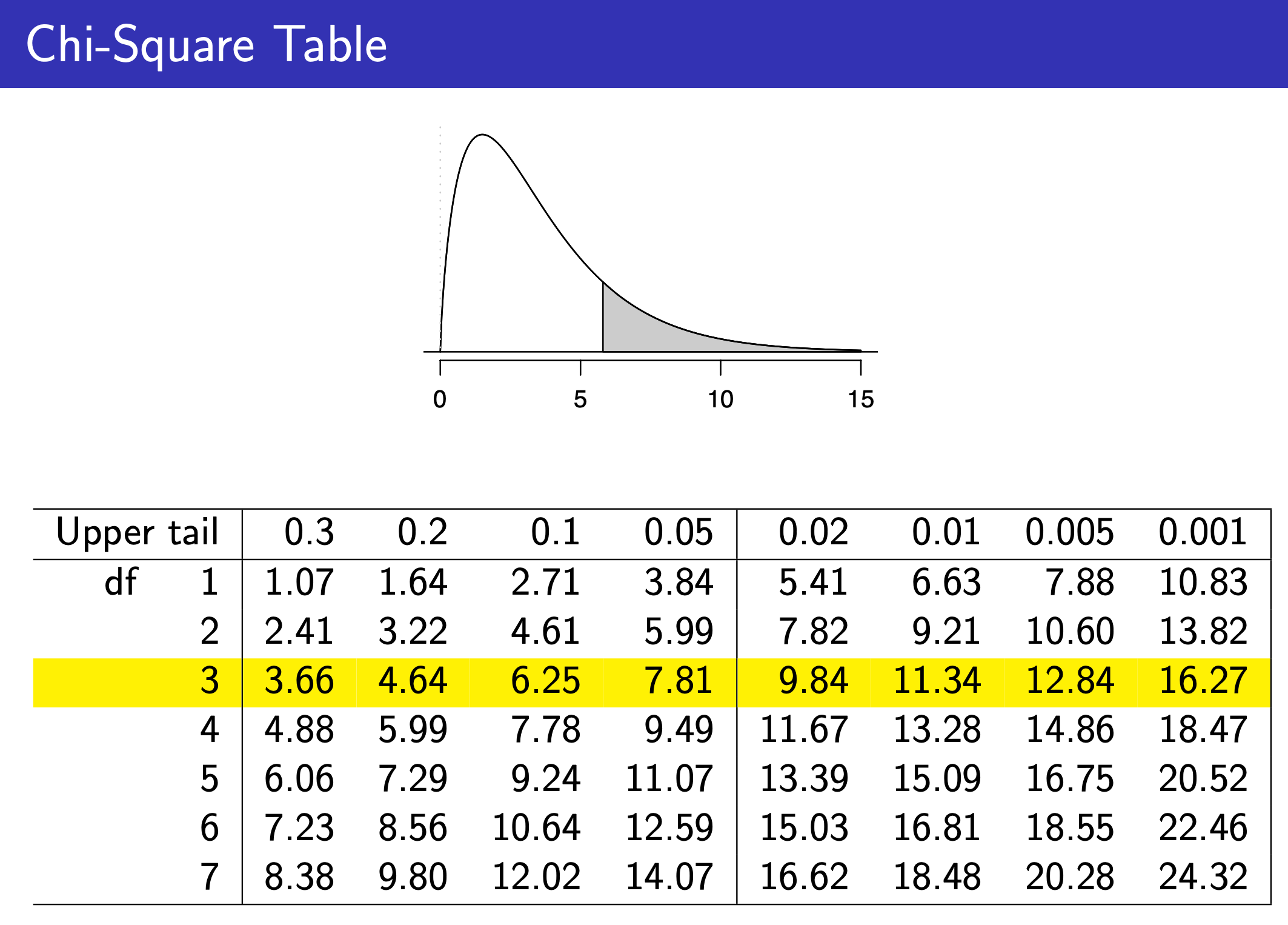
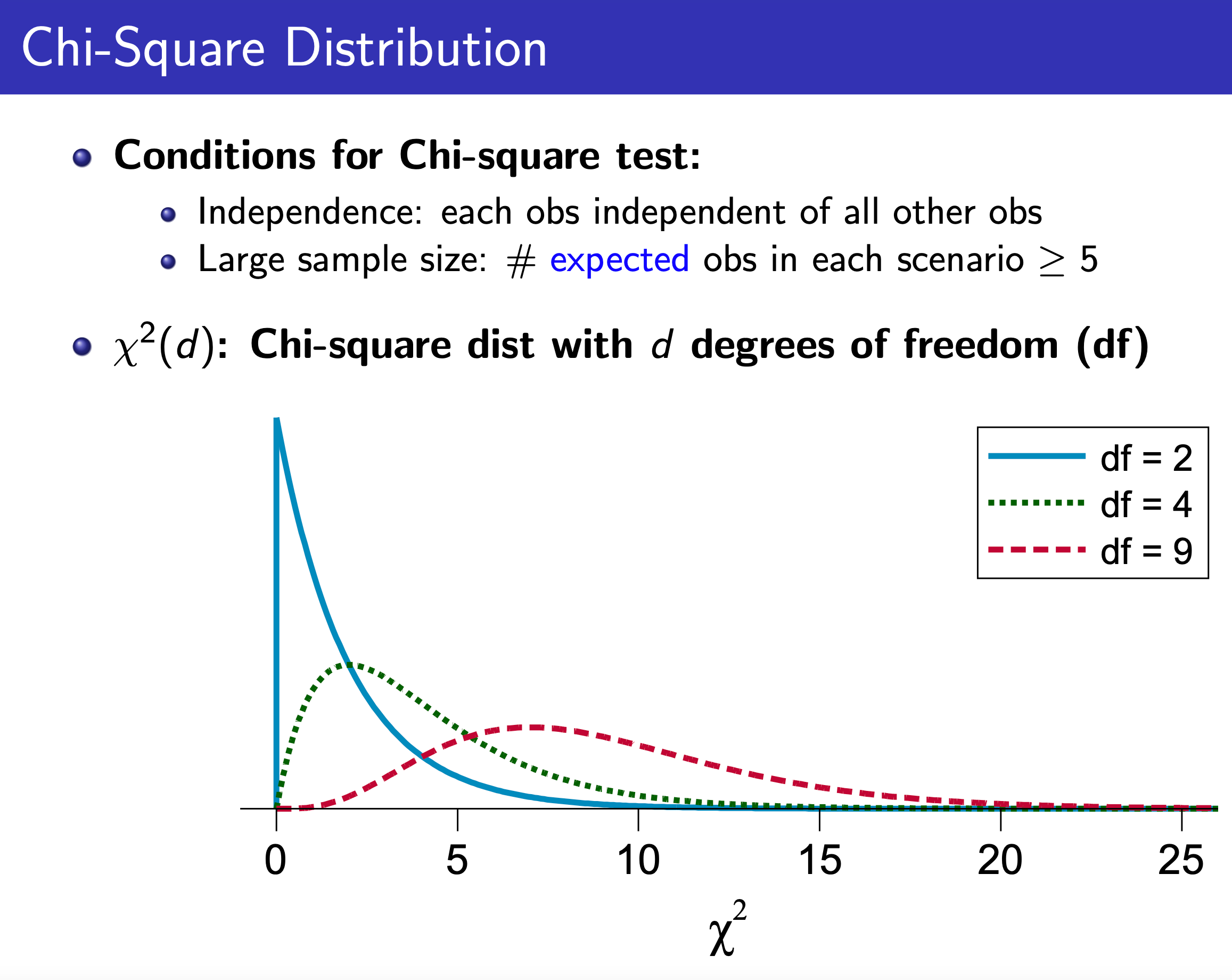
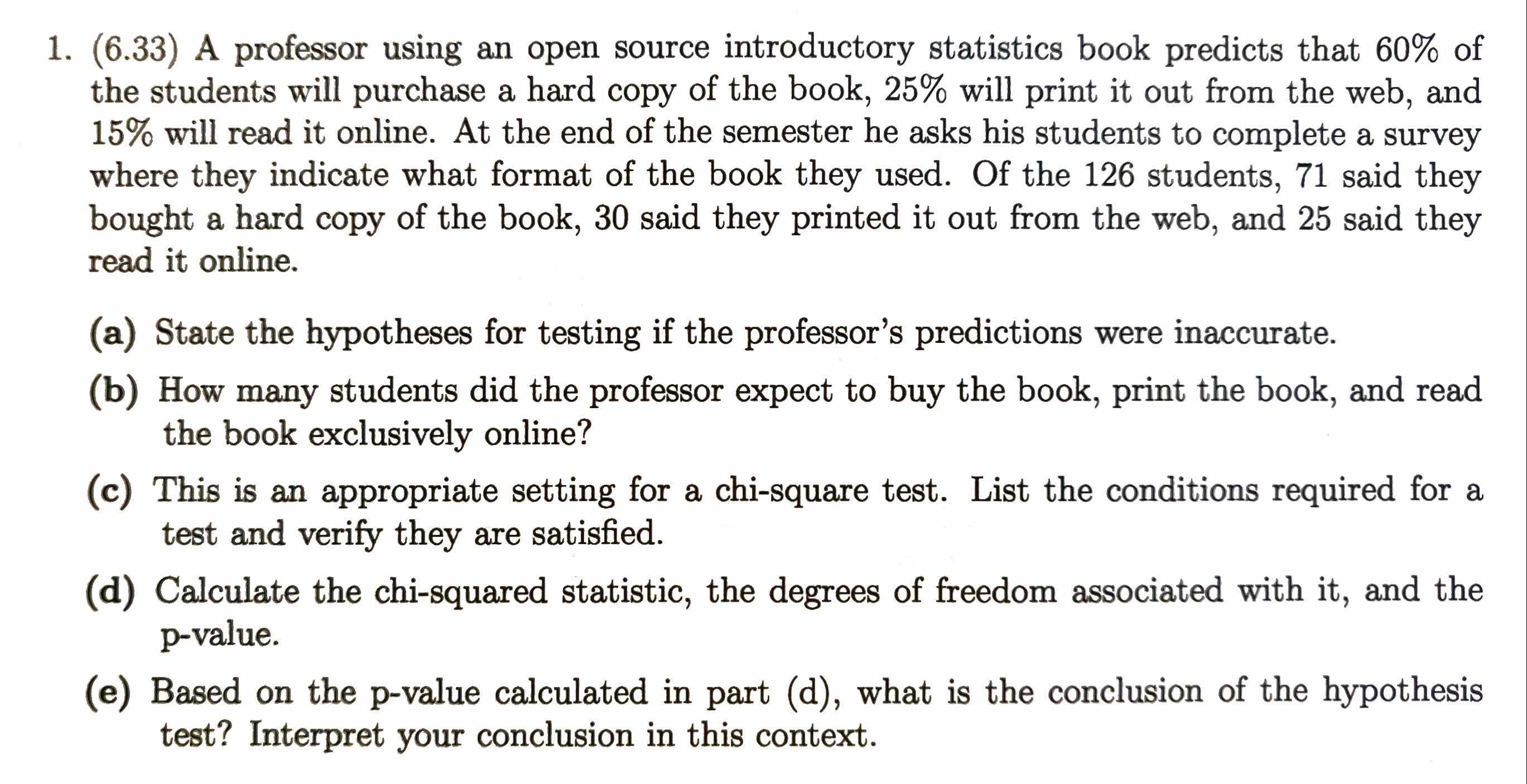
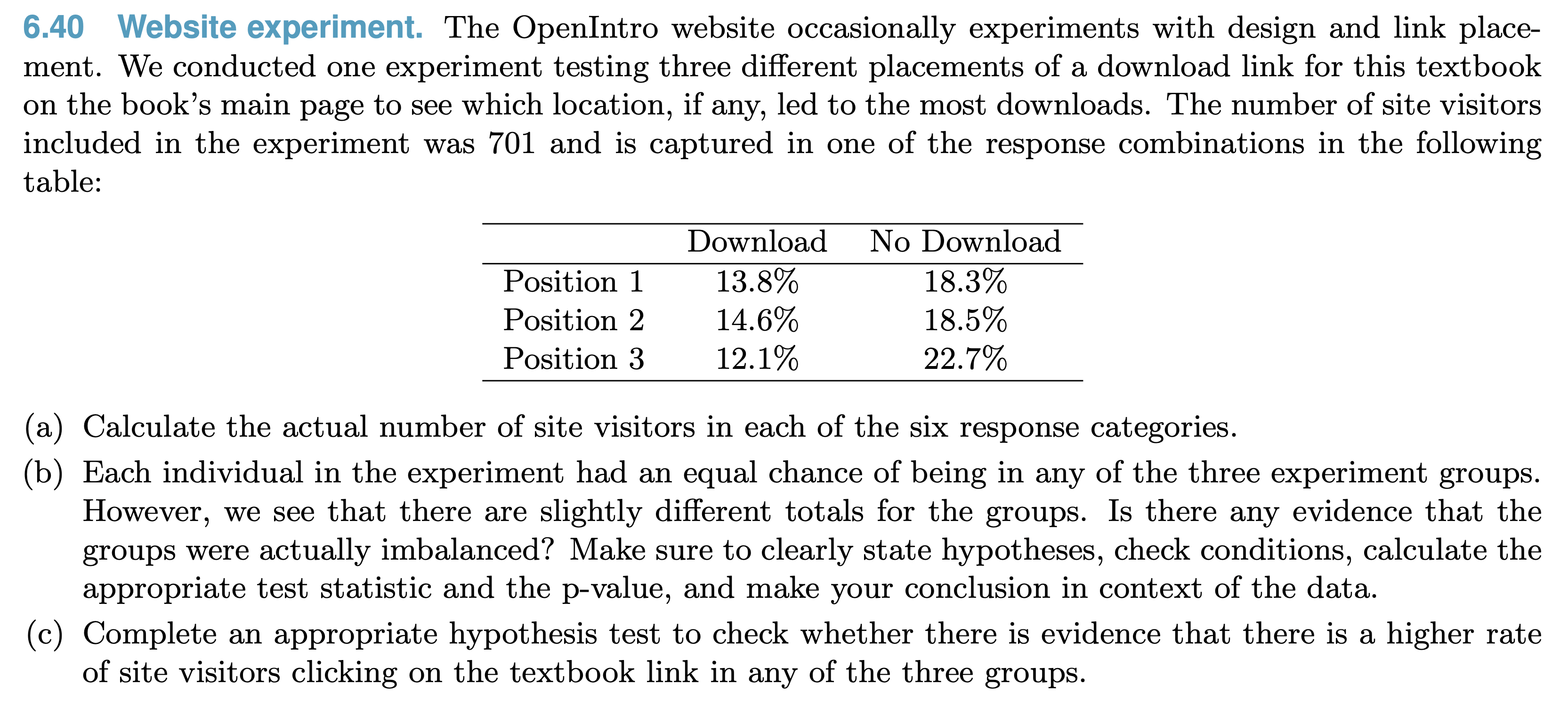
Chi-Square Test¶

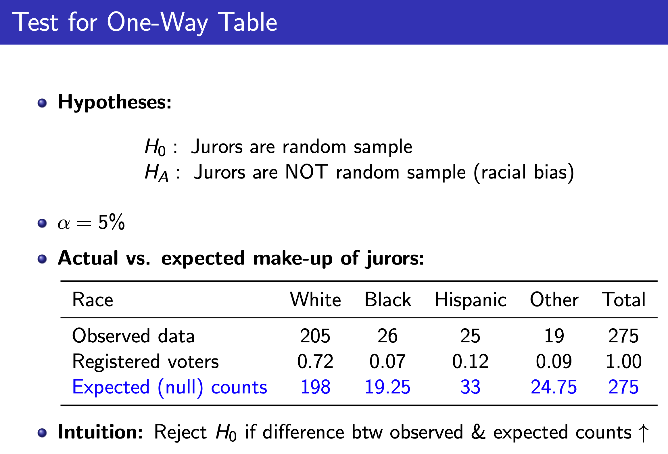
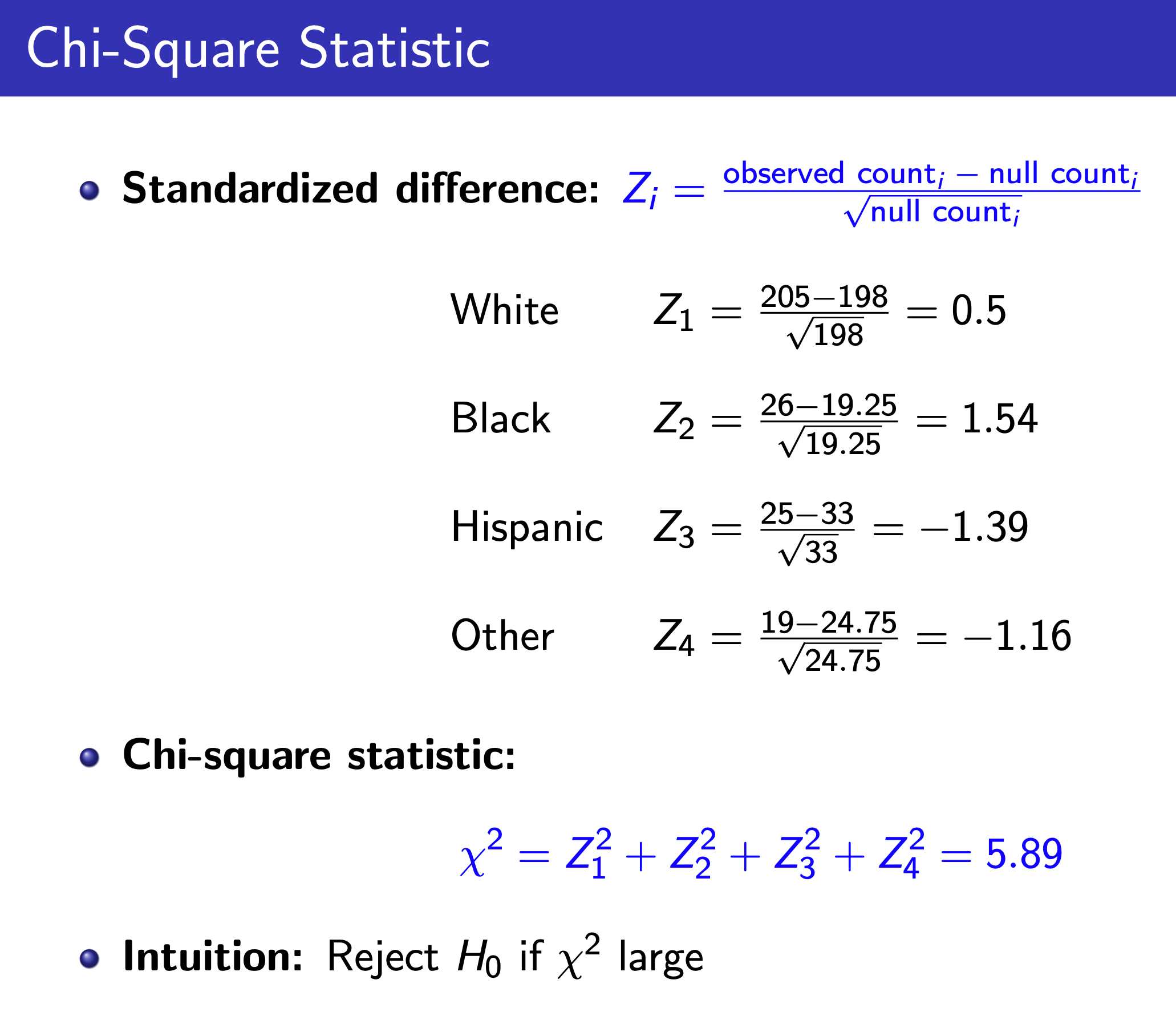
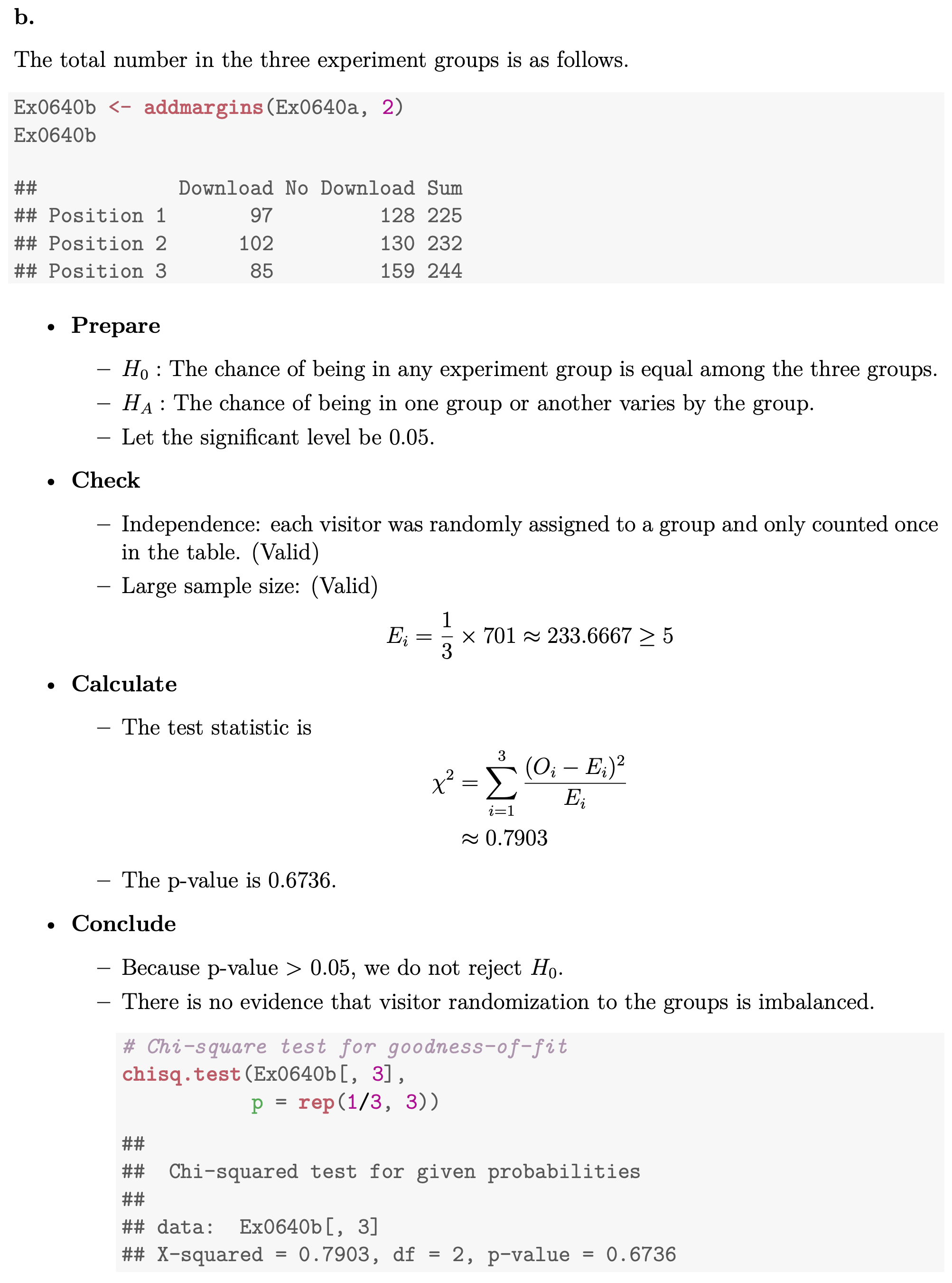
One-Way Table¶

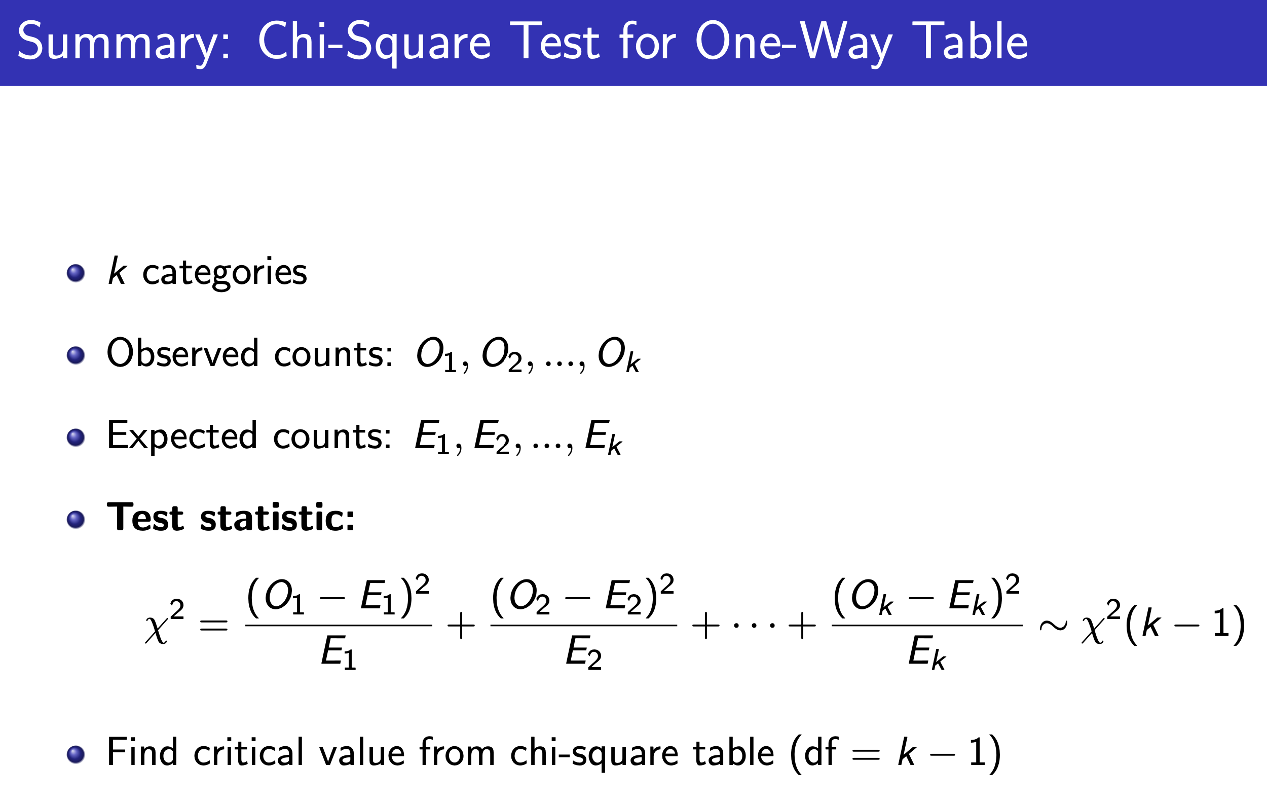
e.g.

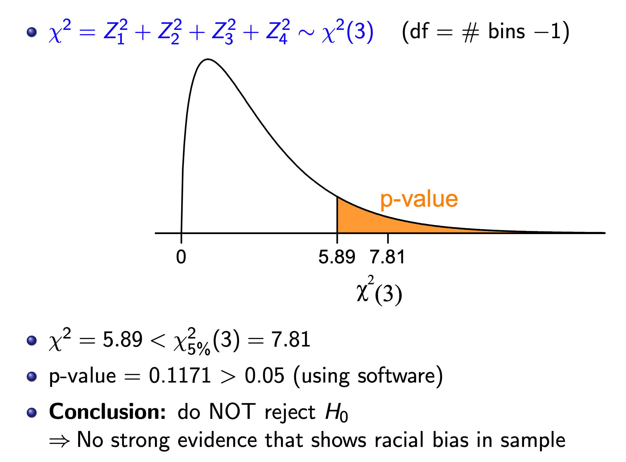
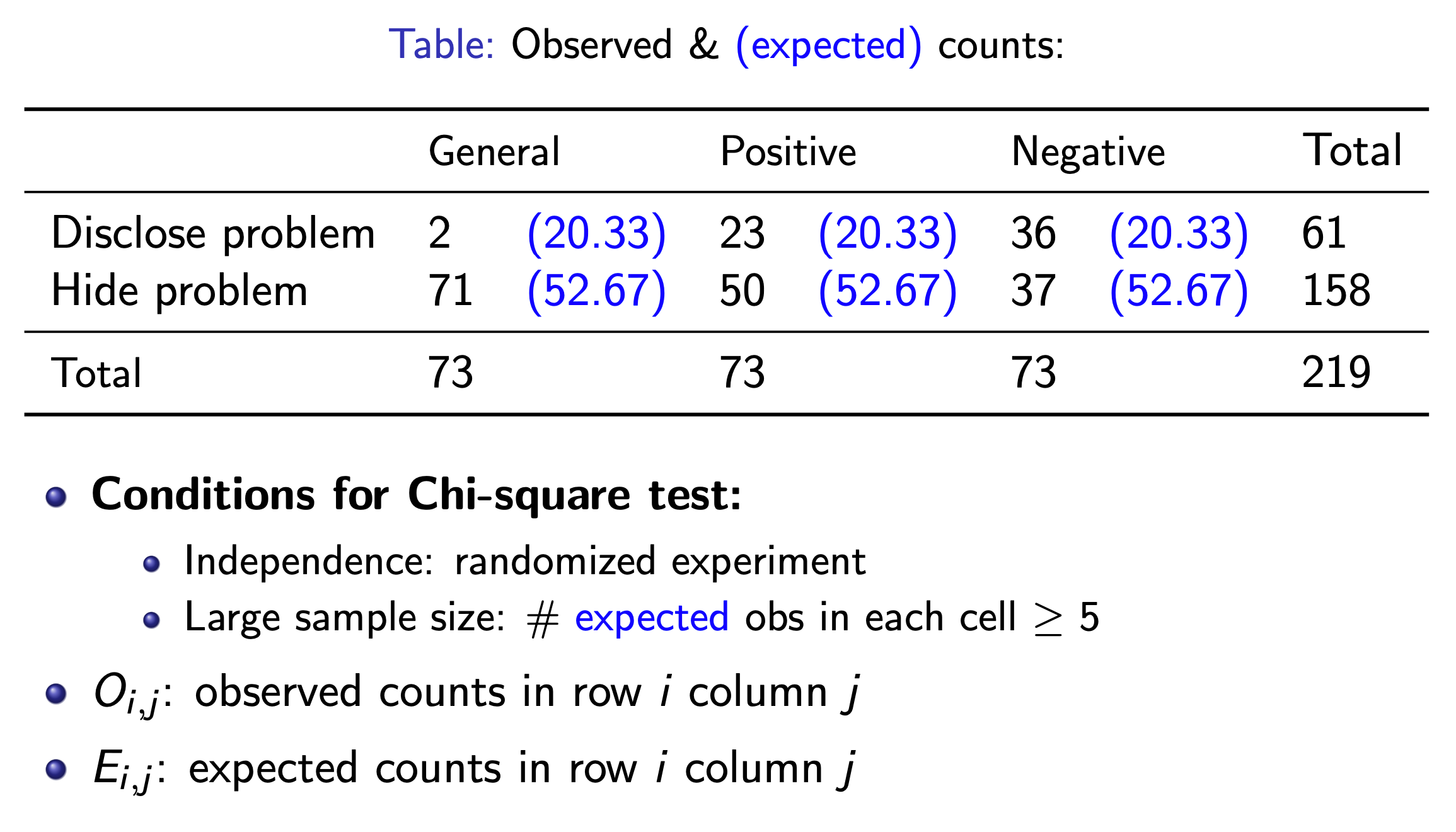
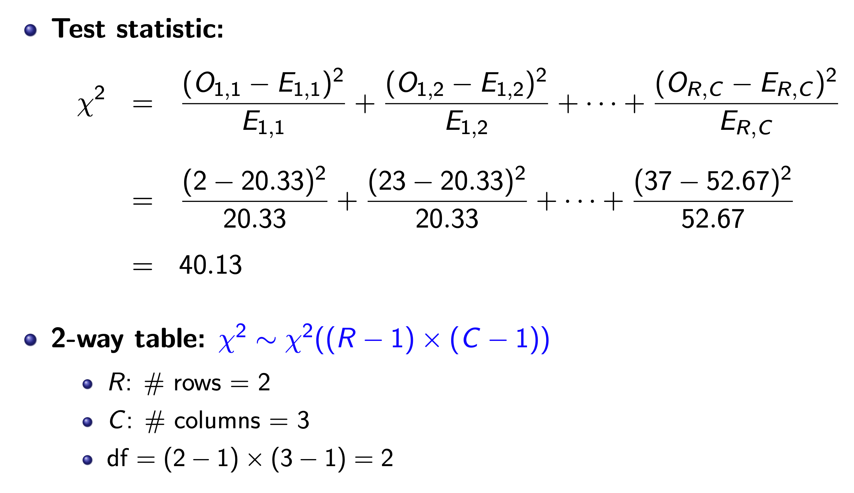
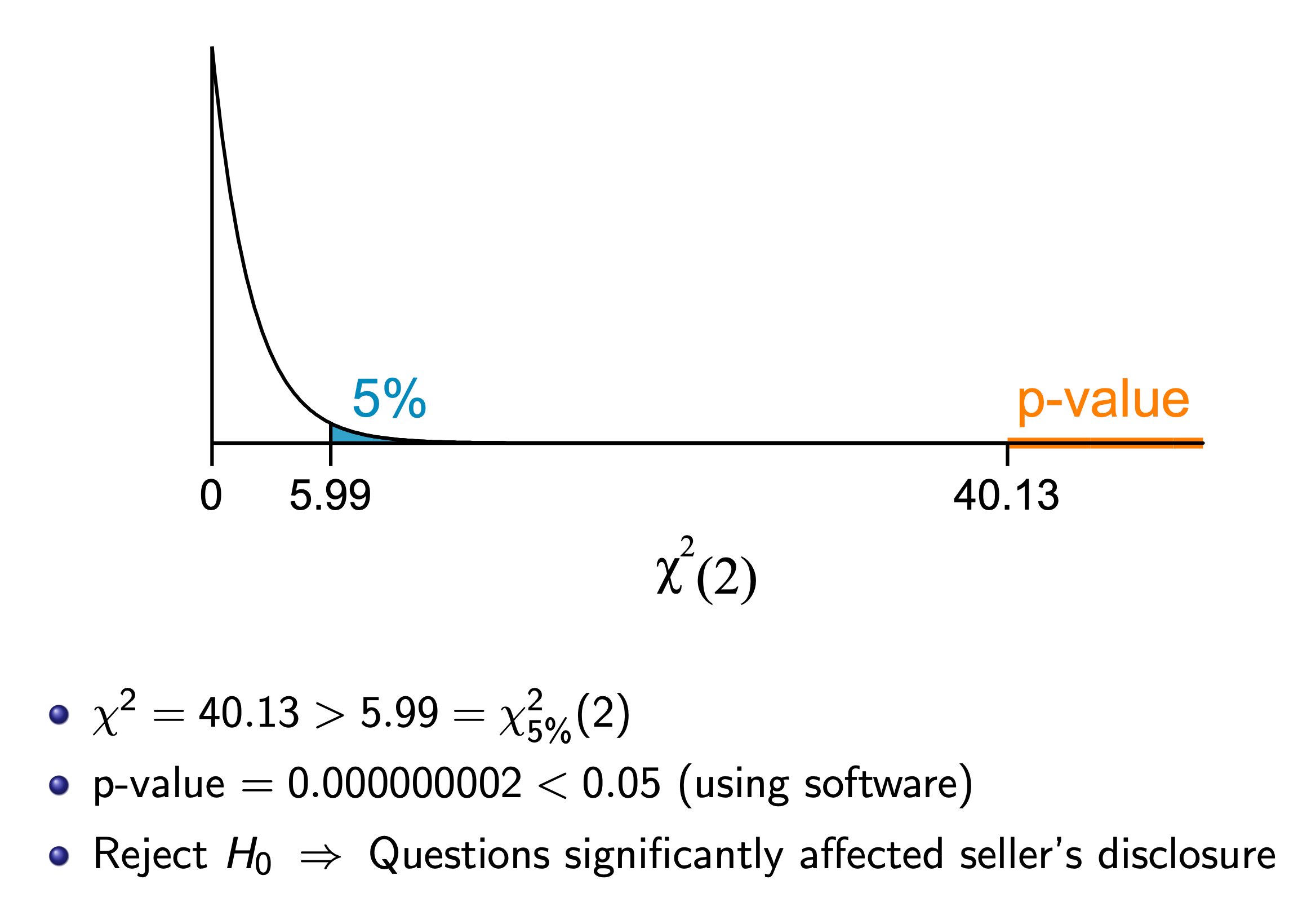
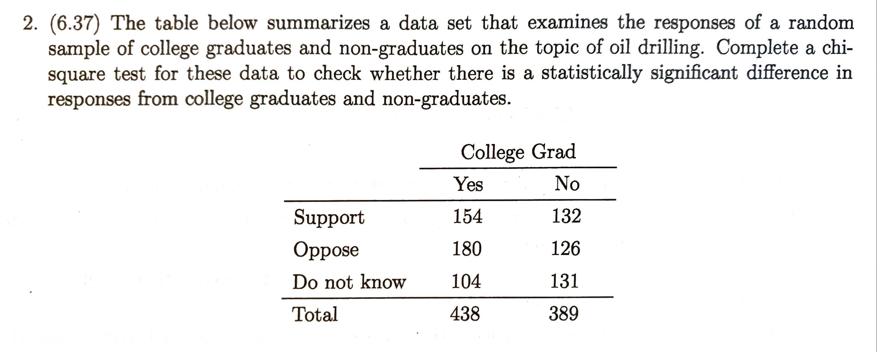
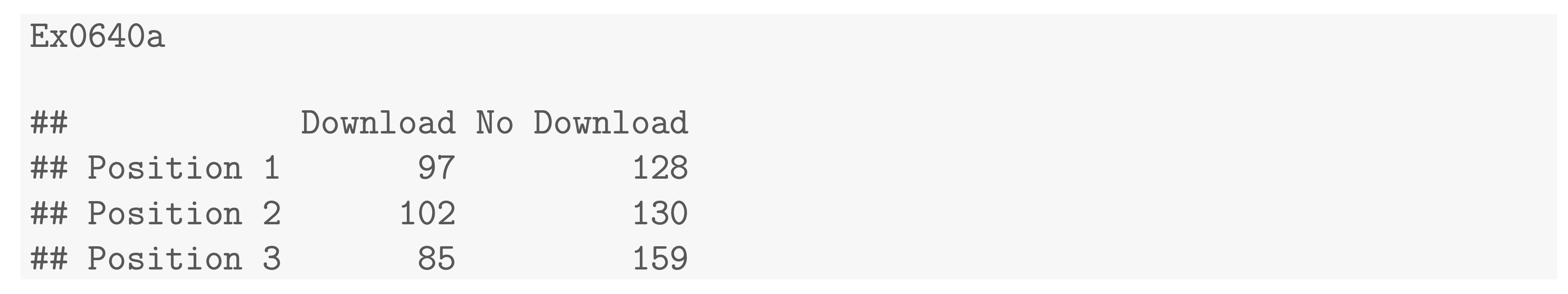
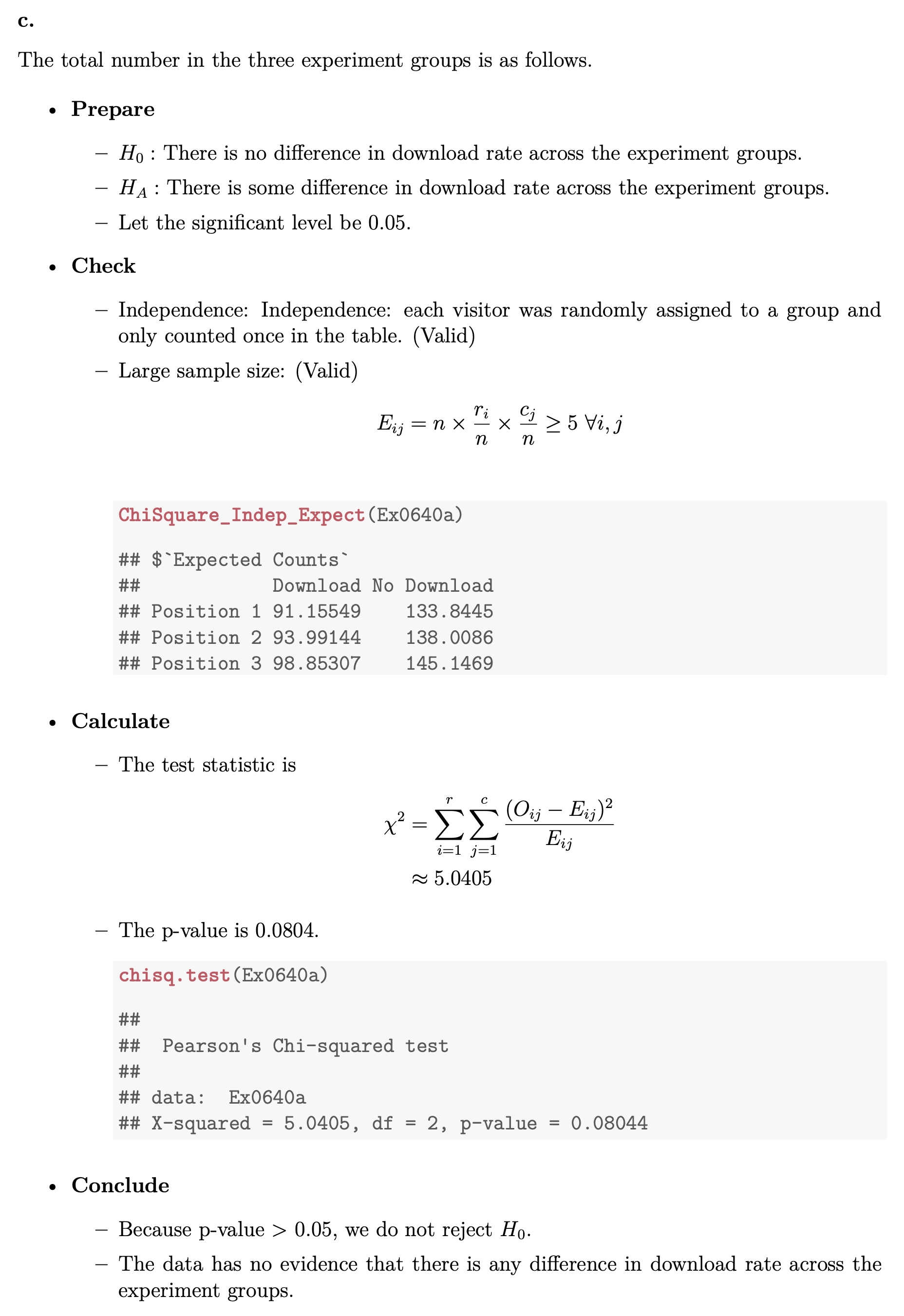
Two-Way Table¶

Each cell is an element, and the caluclate the x square as in one-way table, except df = (# of row - 1)(# of col -1)

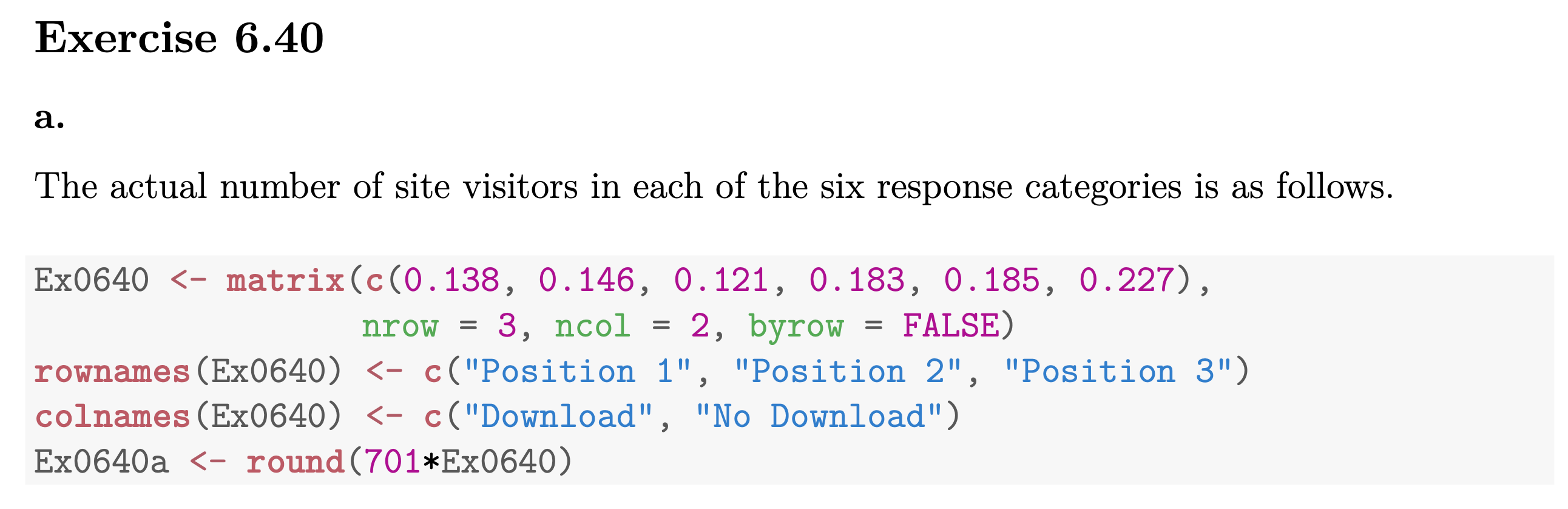
Problems¶

Inference for Numerical Data¶

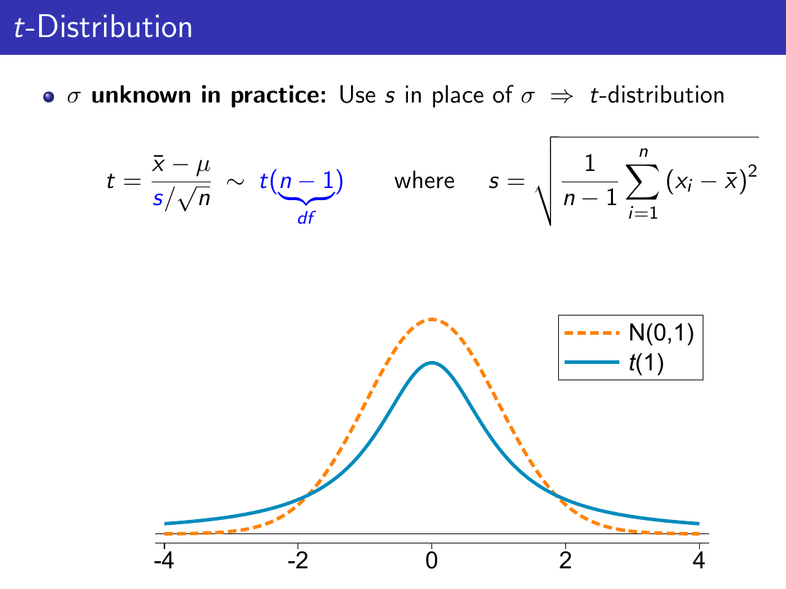
T test¶

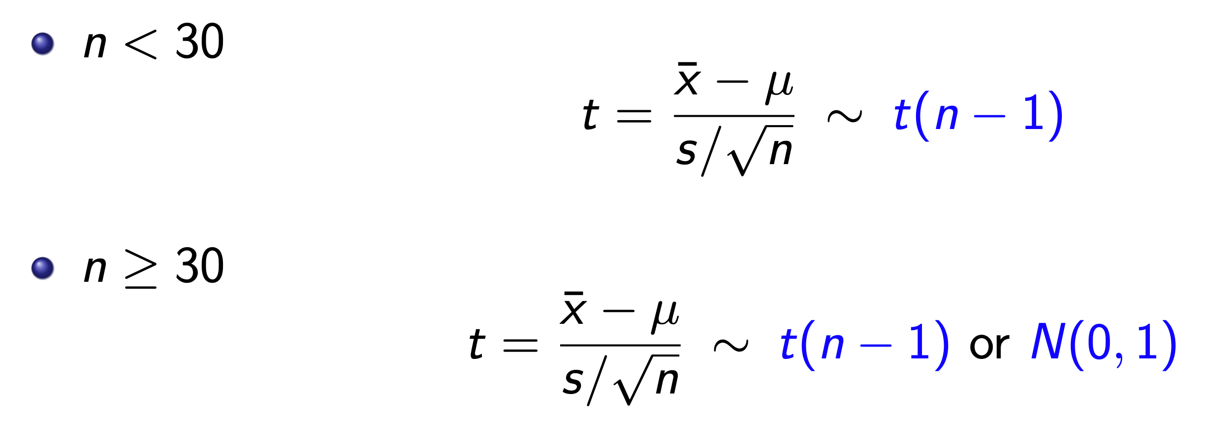
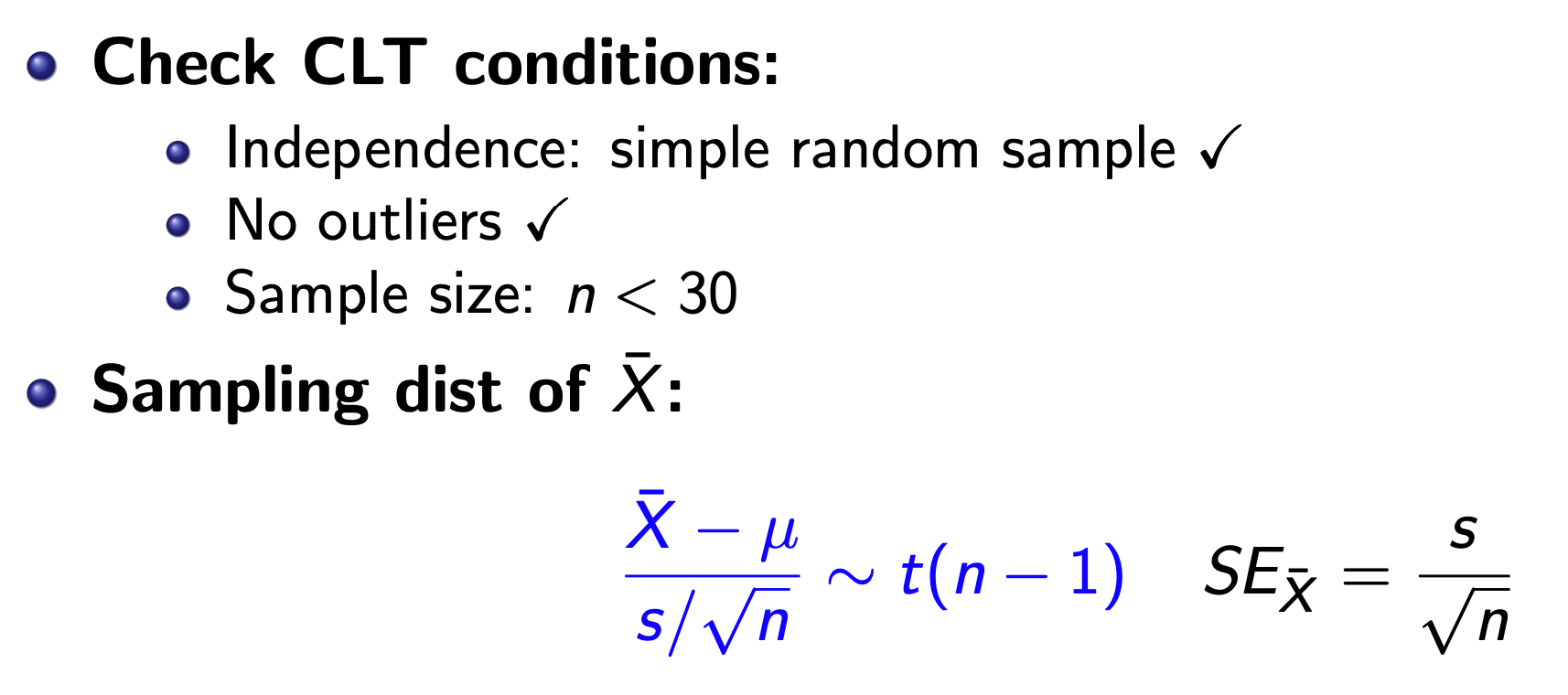
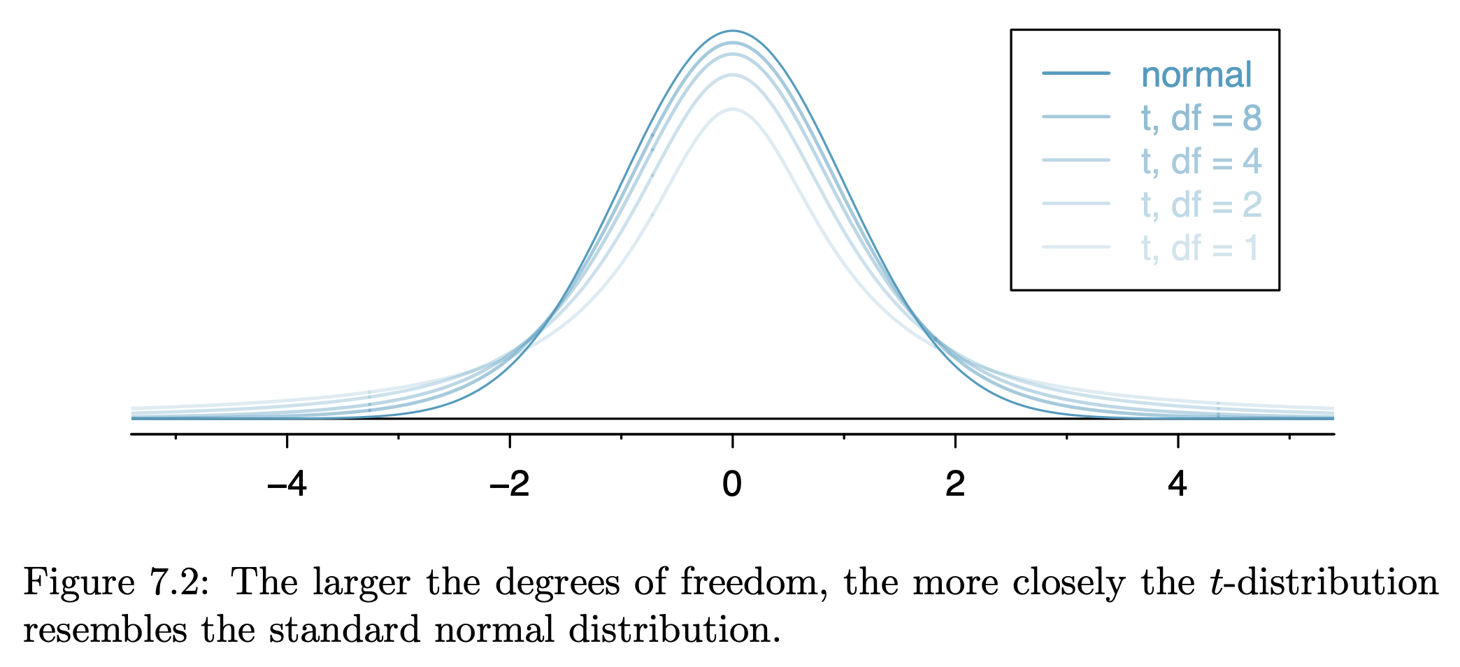
T-Distribution is used when sample size < 30 to solve the problem of sample standard deviation being inaccurate in small samples when using normal distribution to model.

The bigger the degree of freedom = n - 1, the closer it gets to normal distribution.

T Table

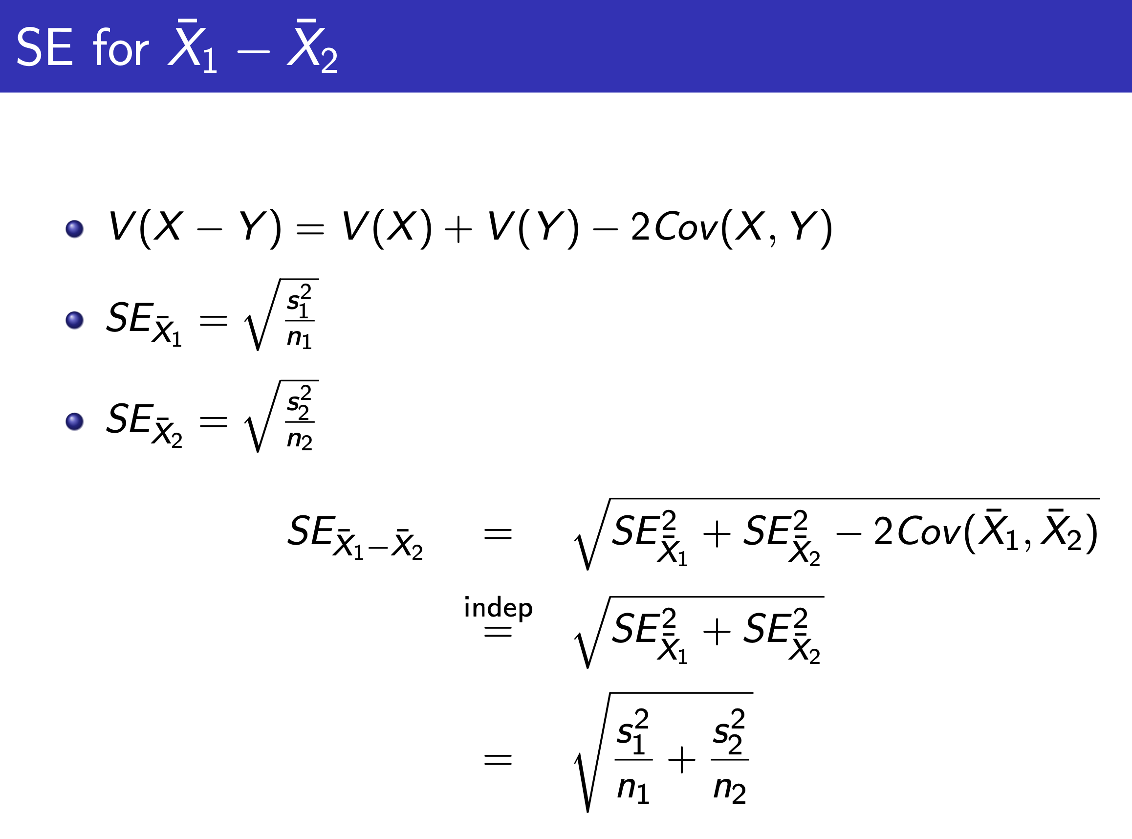
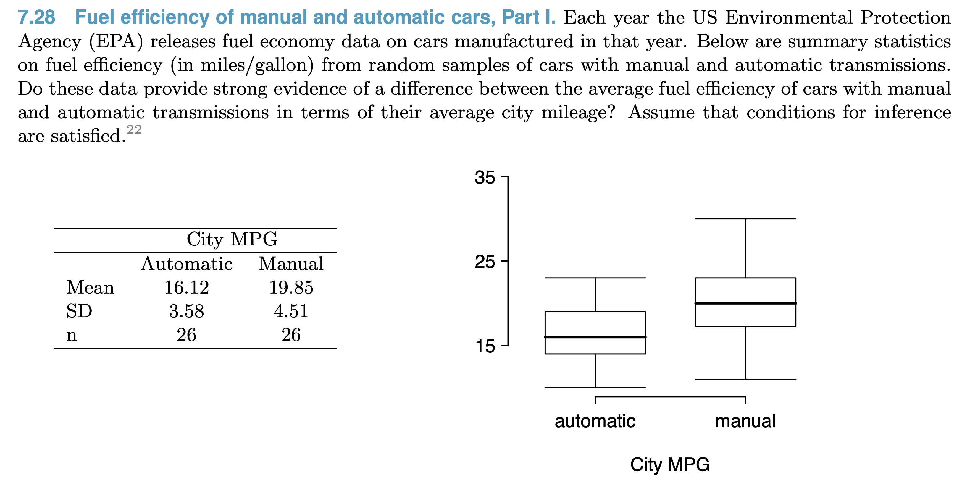
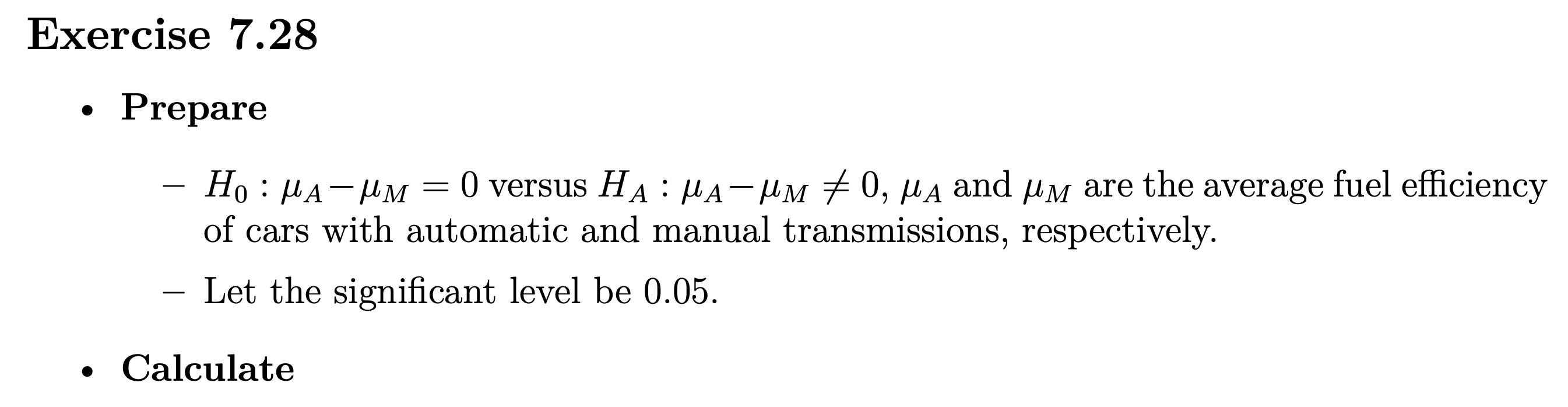
Comparing 2 means

Problem

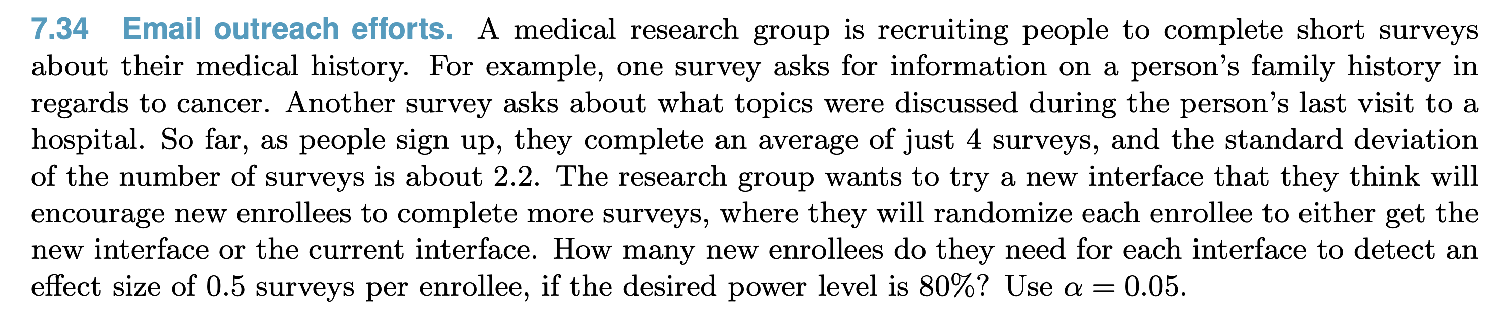
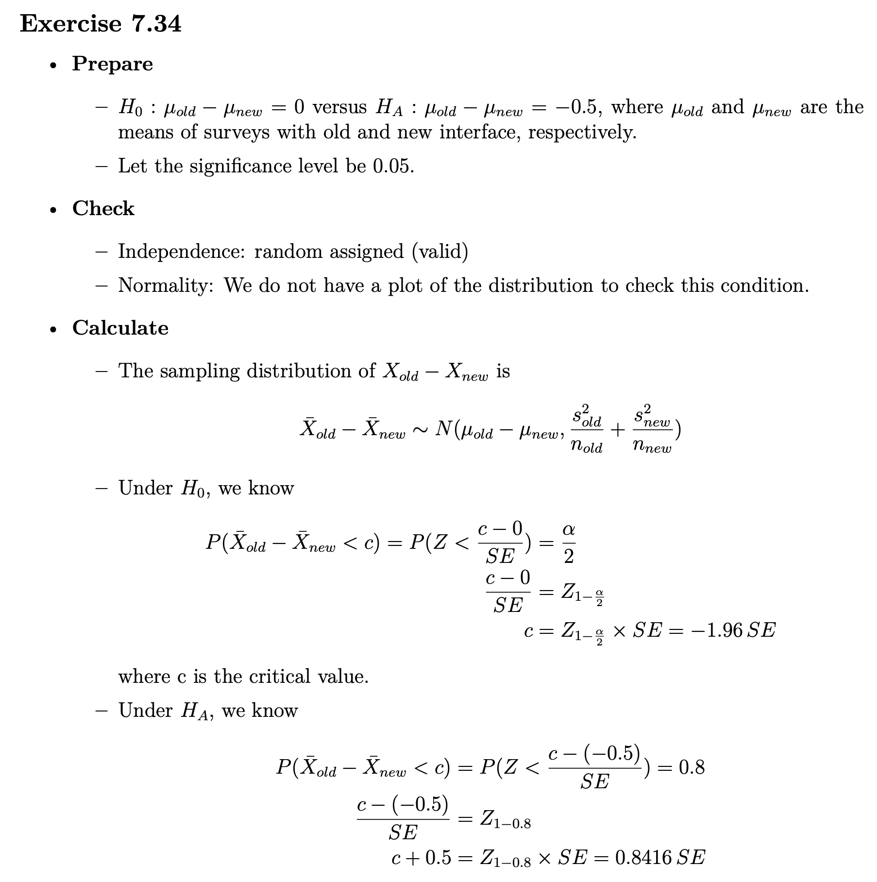
Power of Tests¶

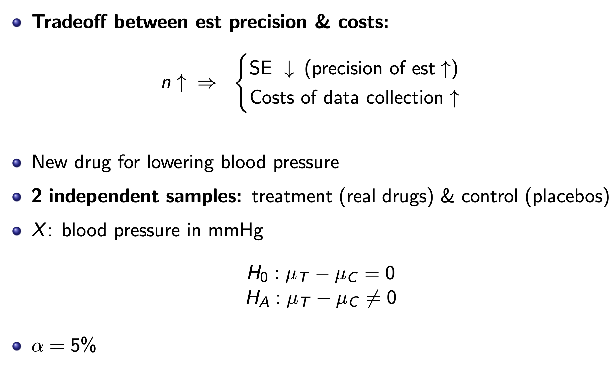
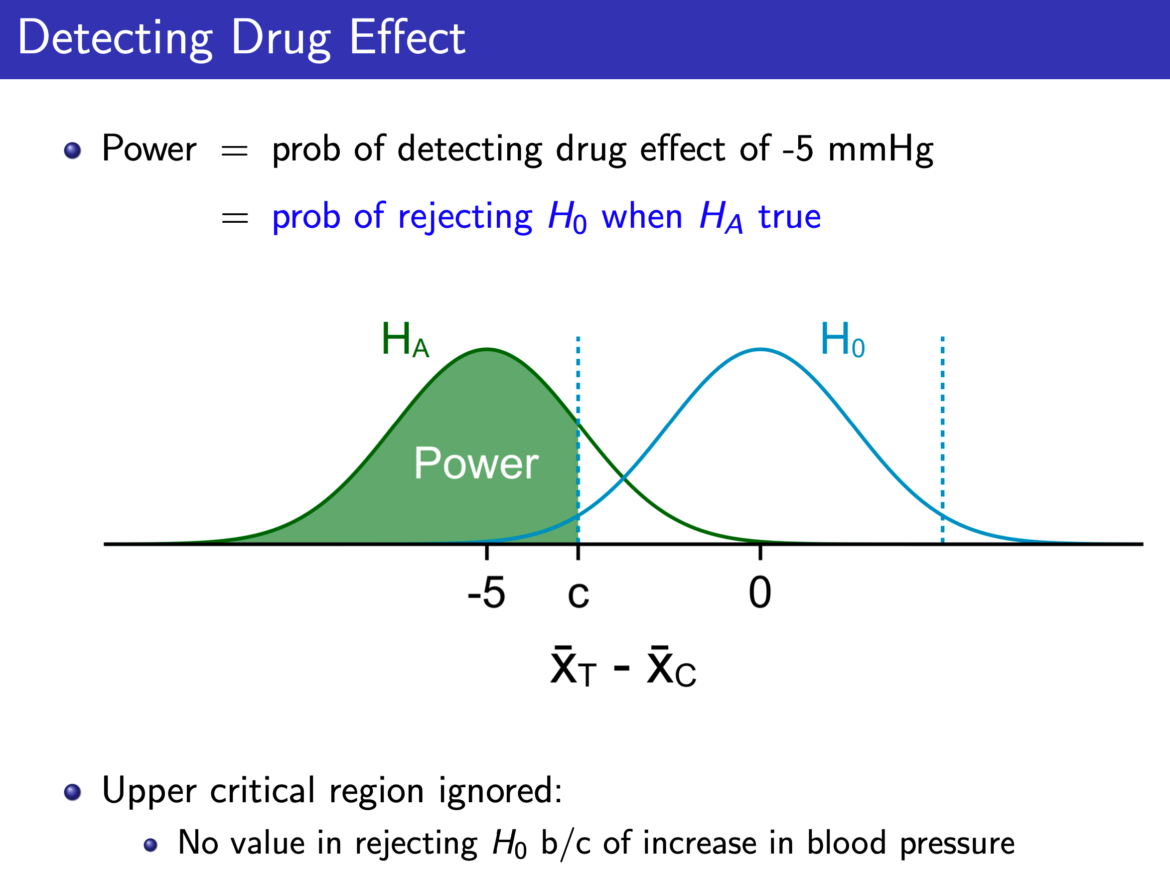
Basically (the Z of power + the Z of the critical value ) x SE = difference of the mean

e.g.

Given
- sample size of both = \(n\)
- \(\mu\)
- SD
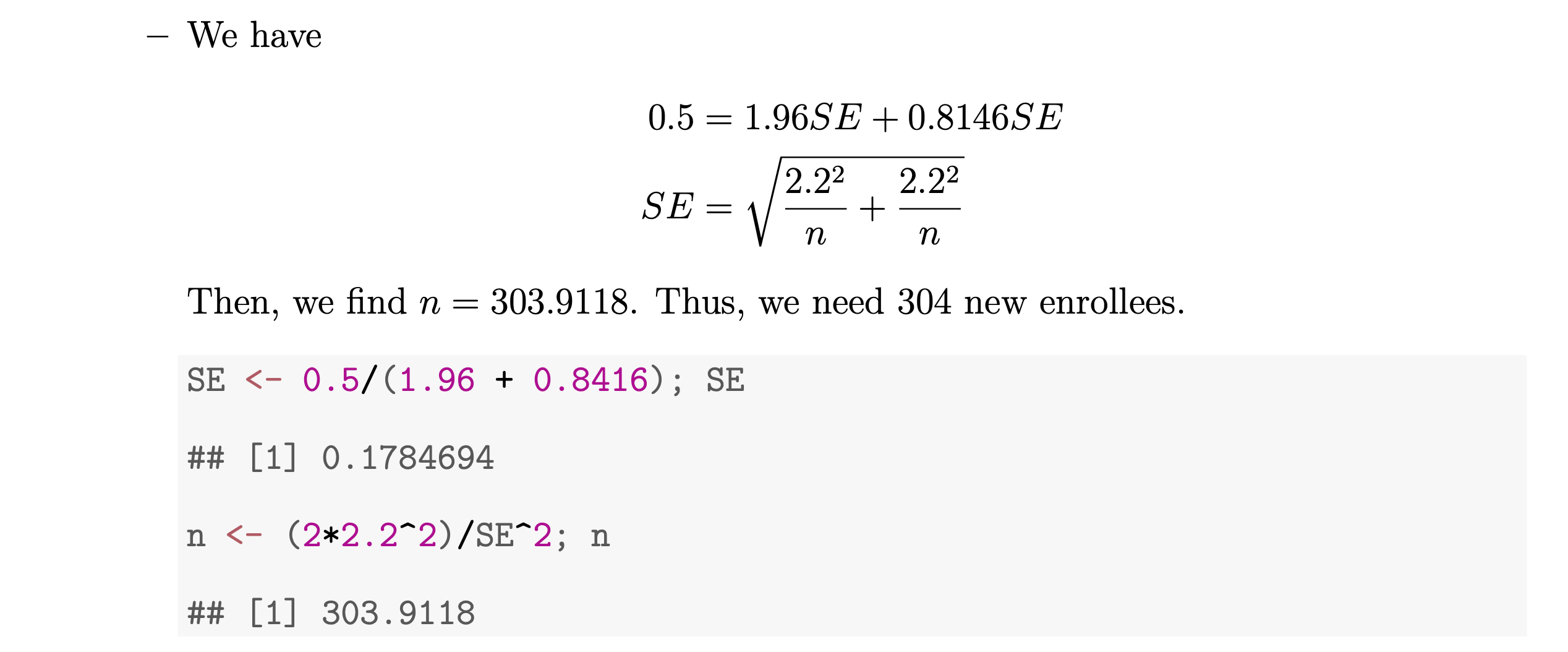
- difference of mean = 0.5
- \(\alpha\) = 5%
  - P(Z<-1.96) = 2.5%
- power = 80%
  - P(Z<0.8416) = 80%
Sol
- SE=\(\sqrt{\dfrac{SD^2}{n}+\dfrac{SD^2}{n}}\)
- (1.96+0.8416)xSE = 0.5
- See graph

Problem

Comparing Means¶

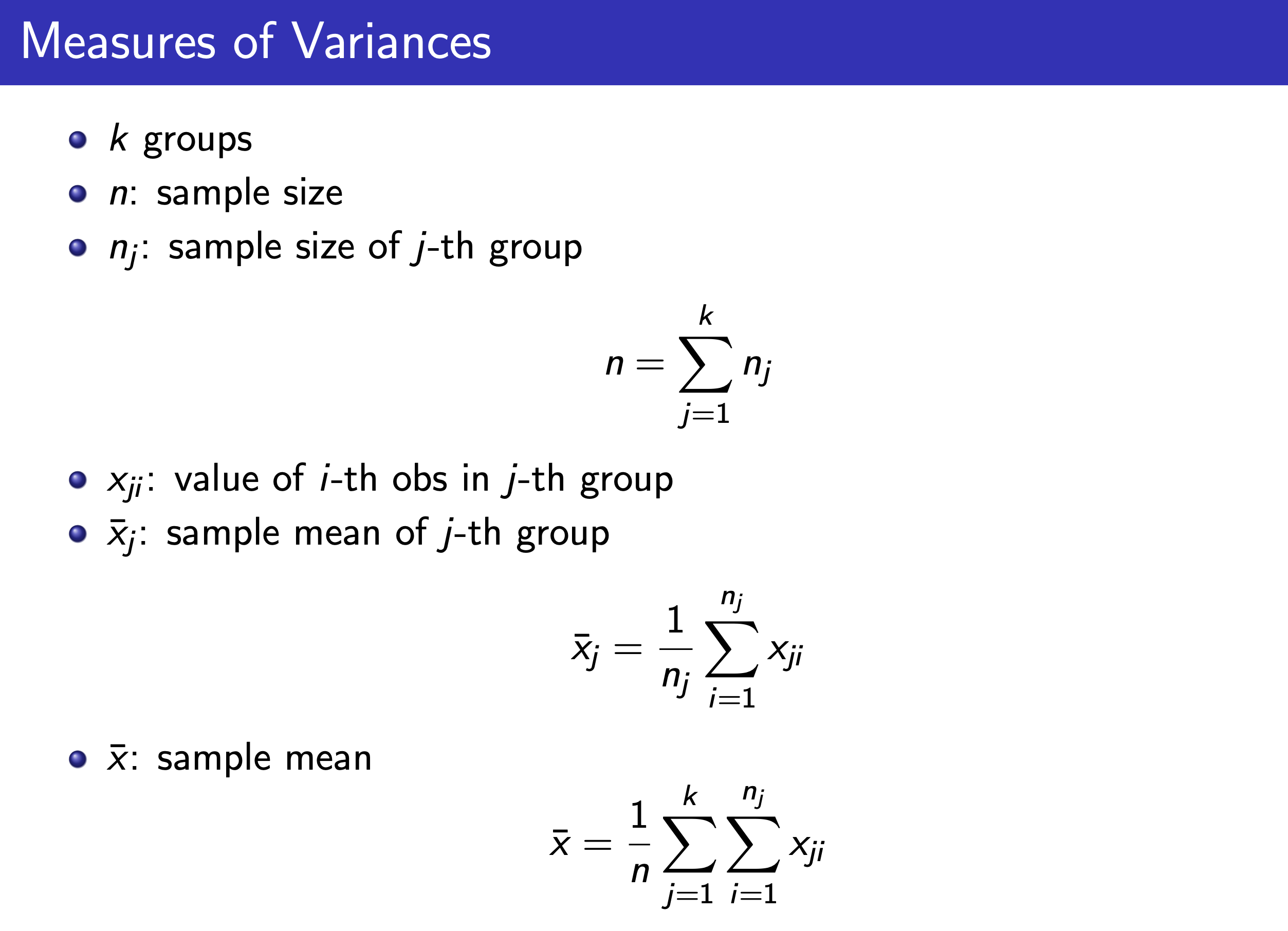
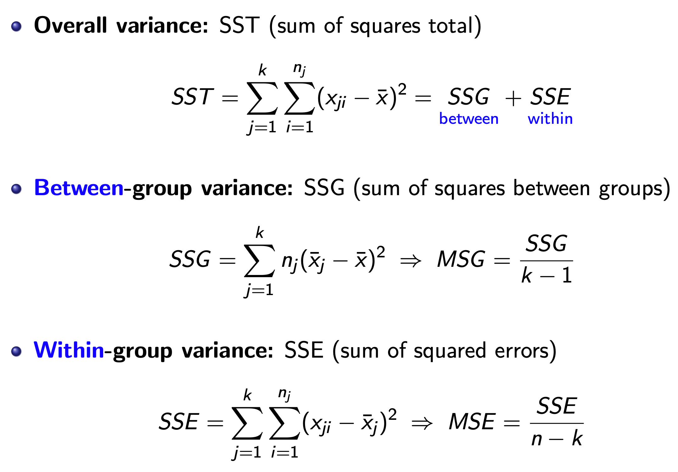
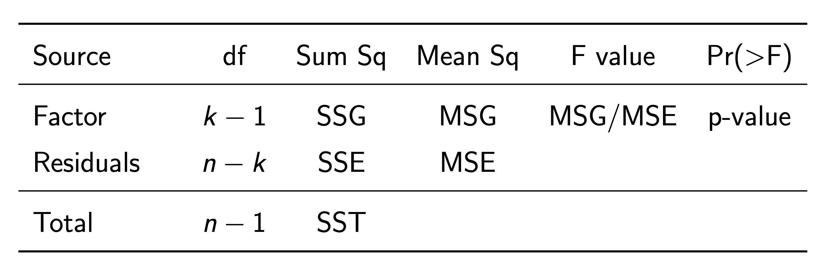
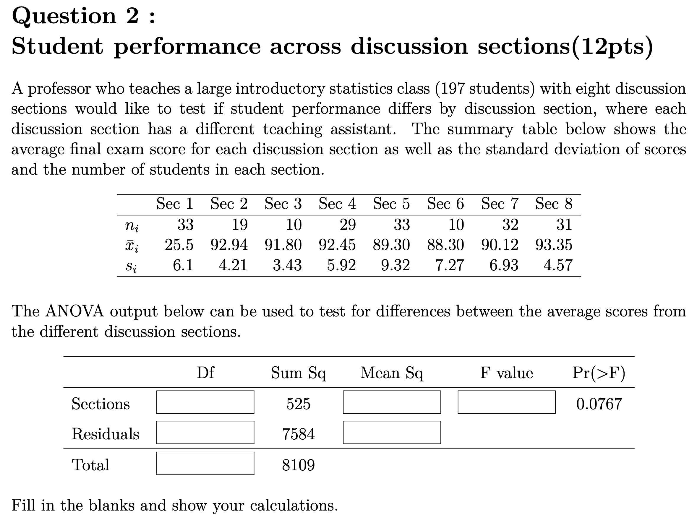
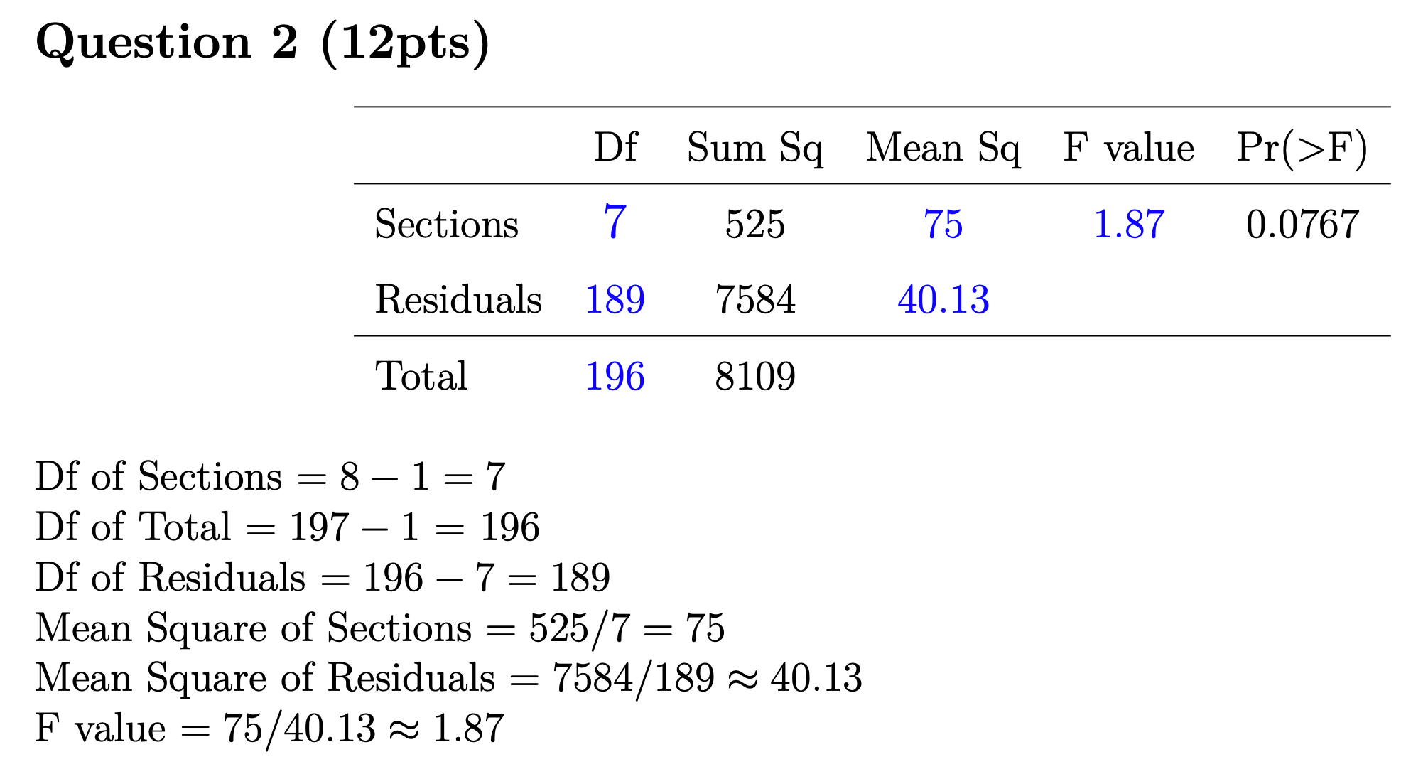
ANOVA & F Test¶

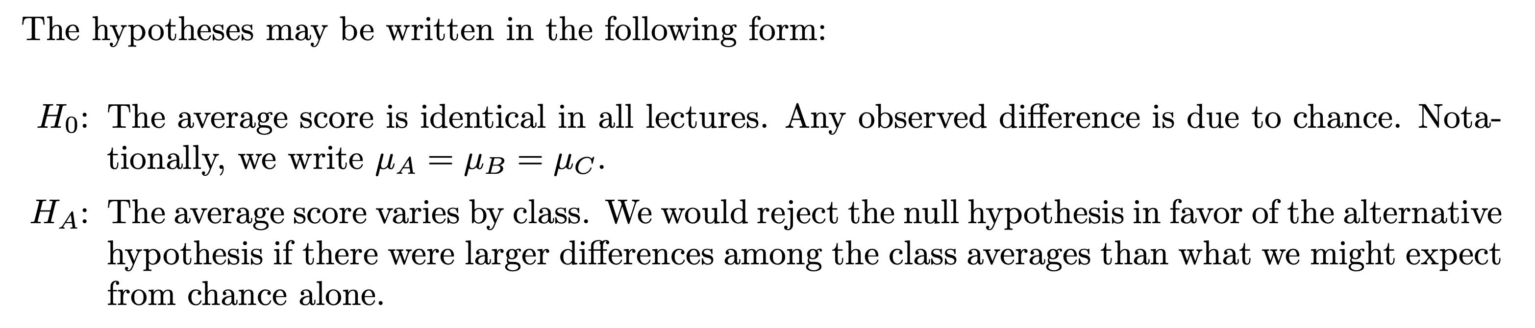
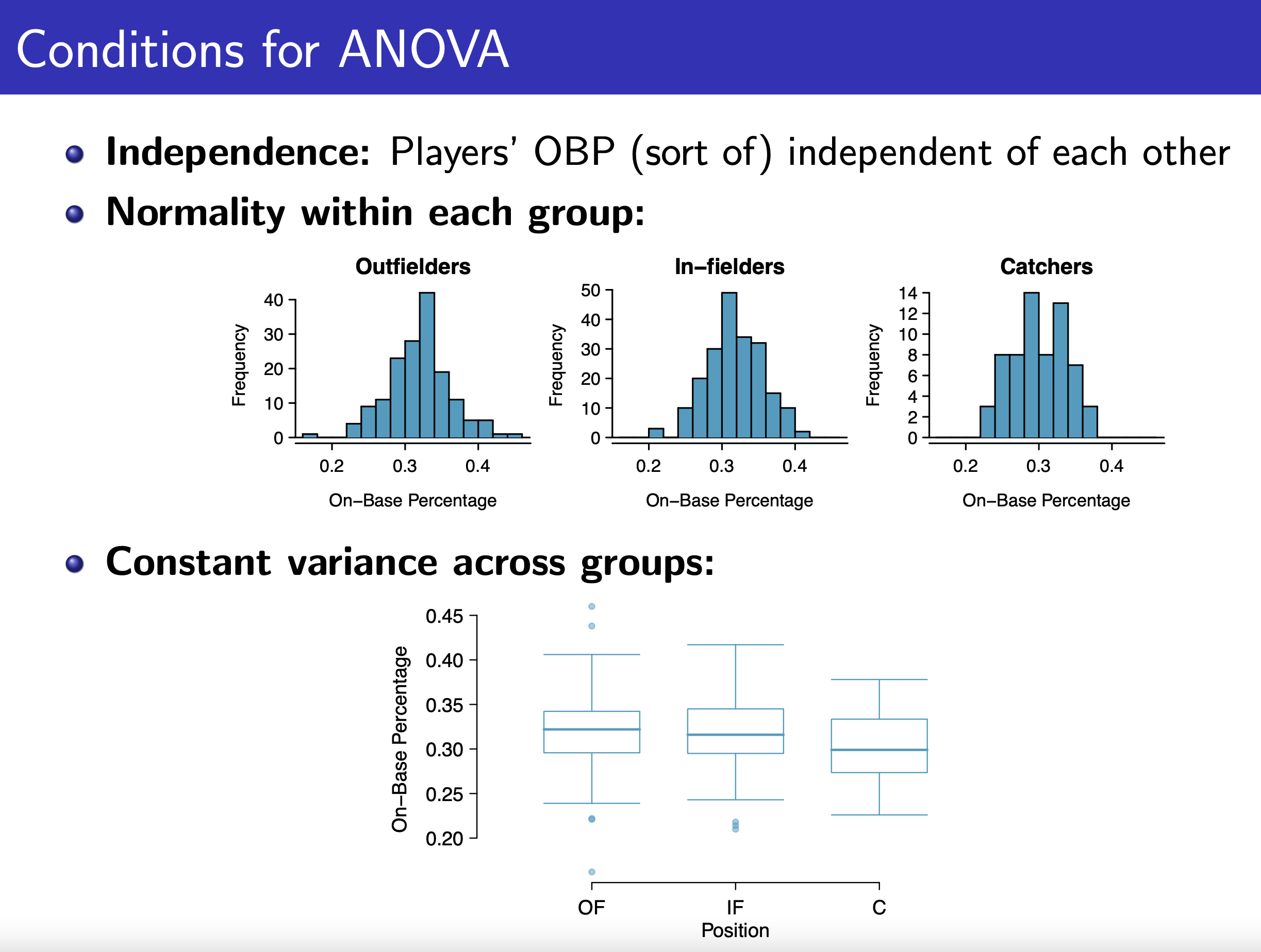
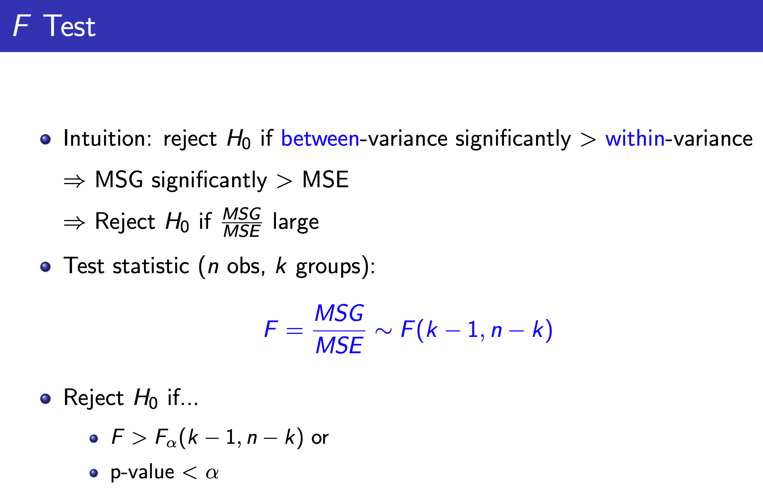
ANOVA Table

Problem

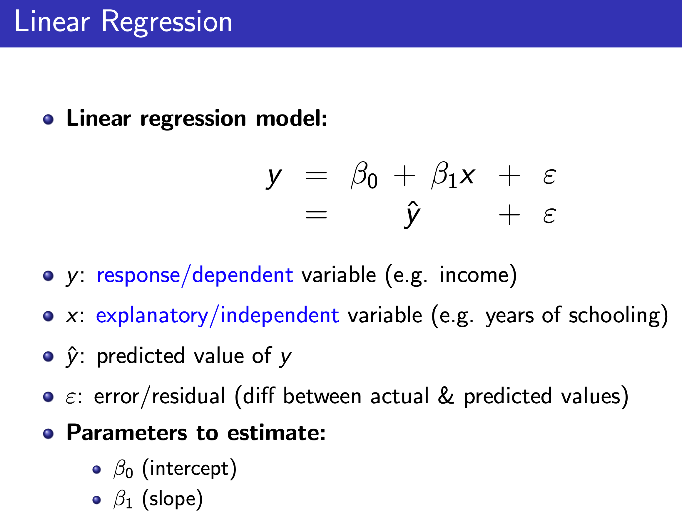
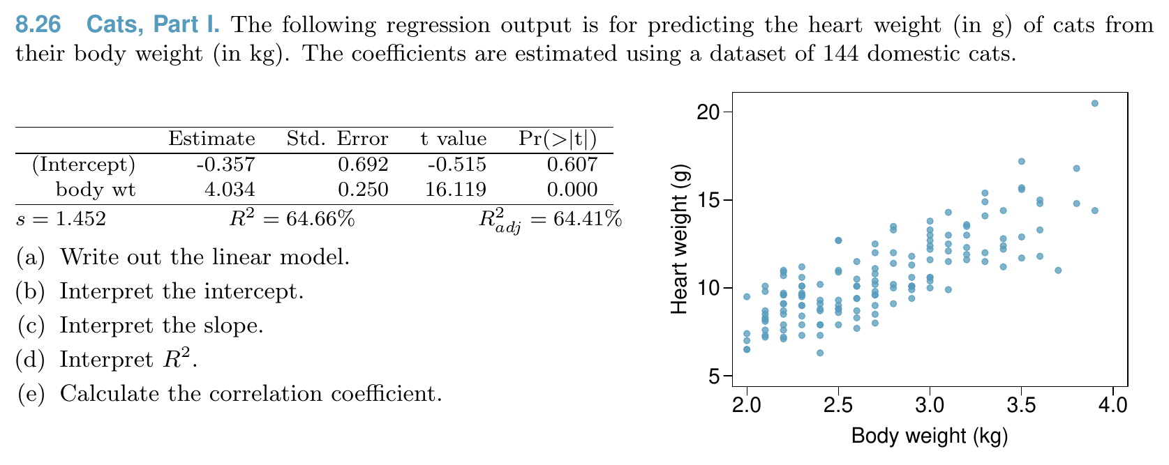
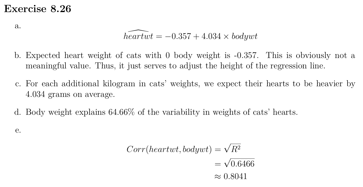
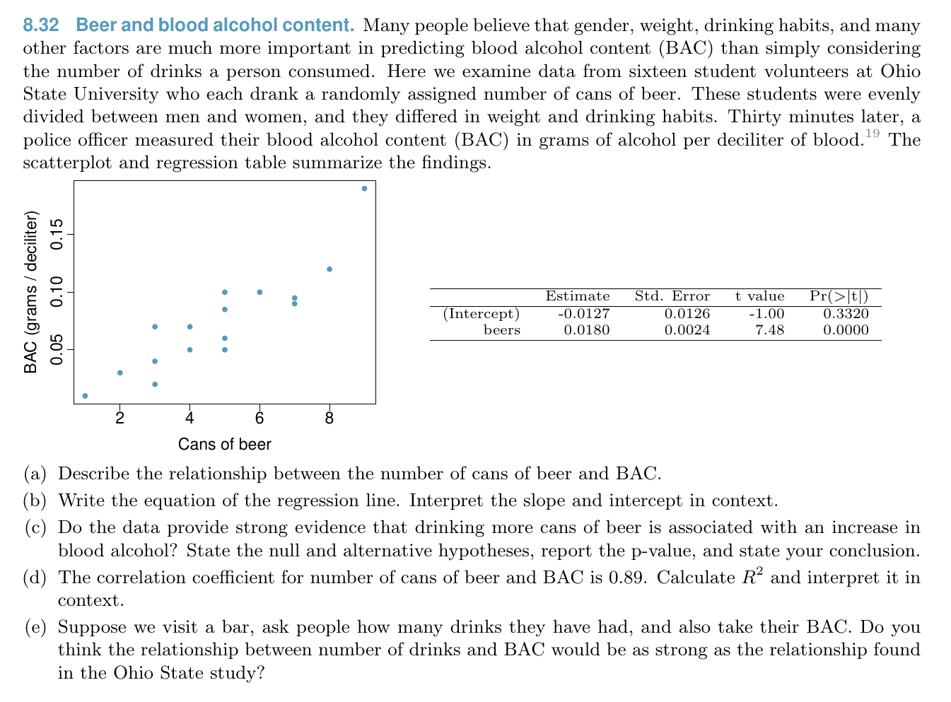
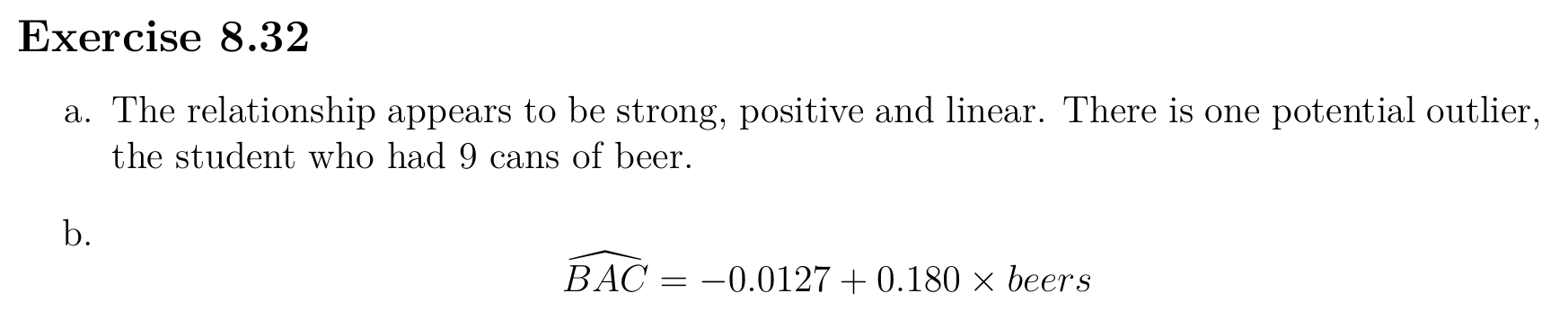
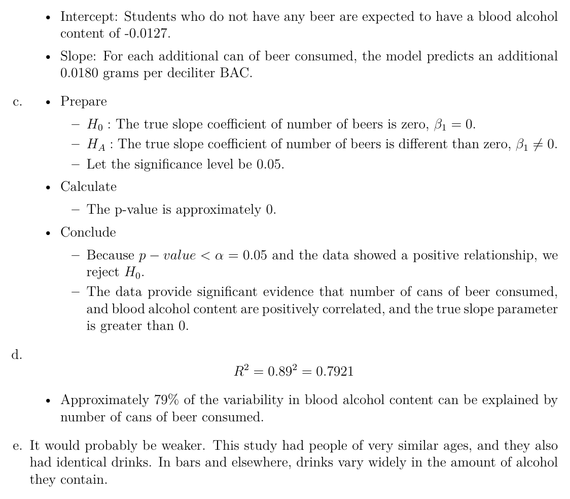
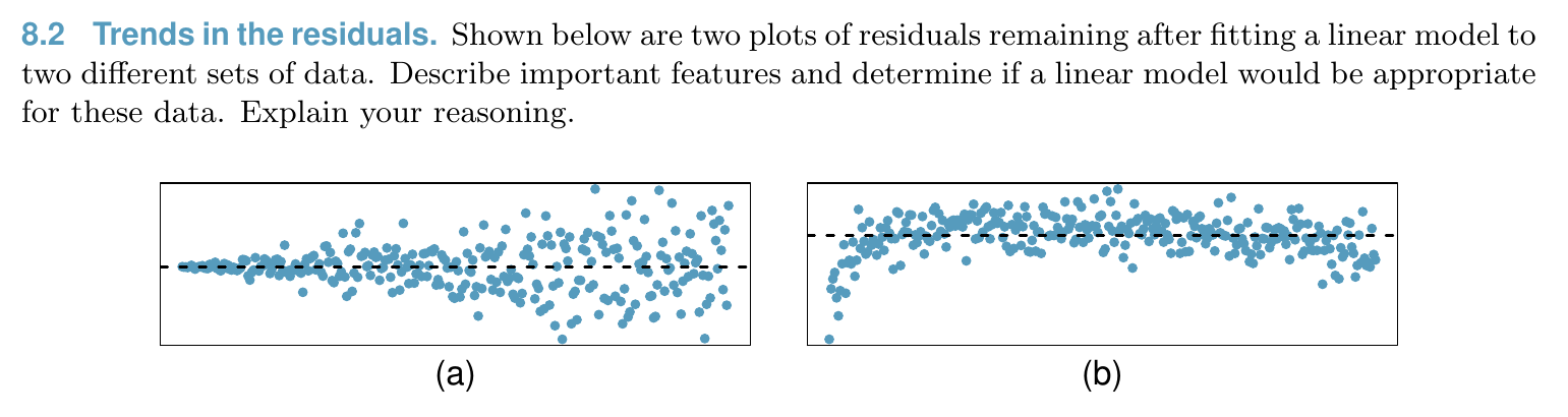
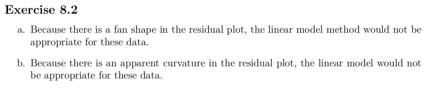
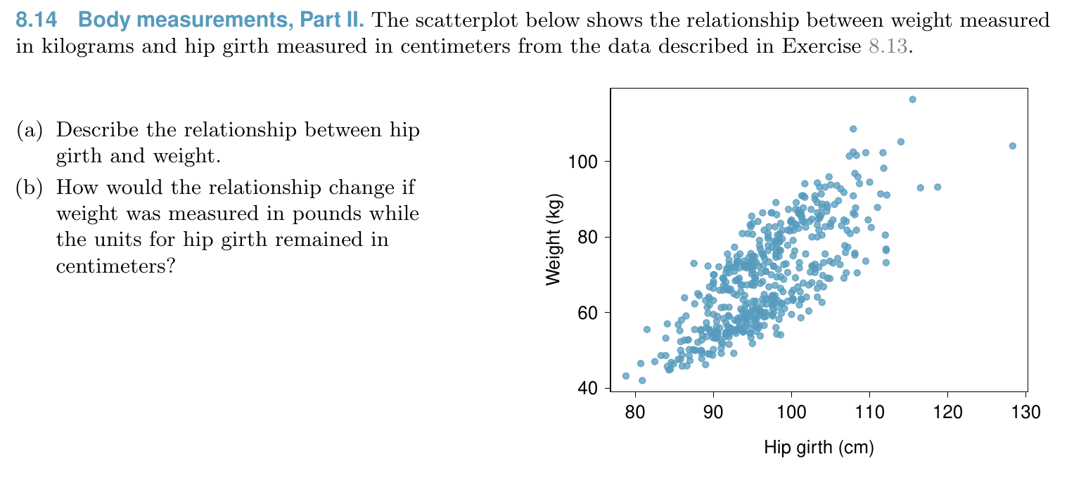
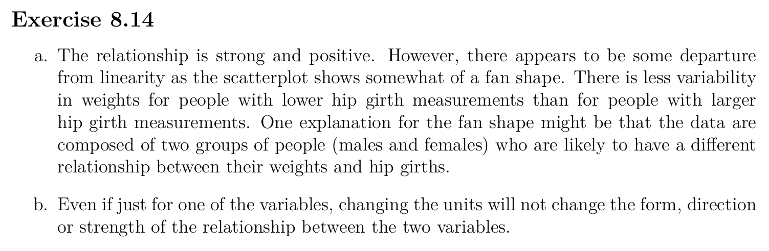
Linear Regression¶

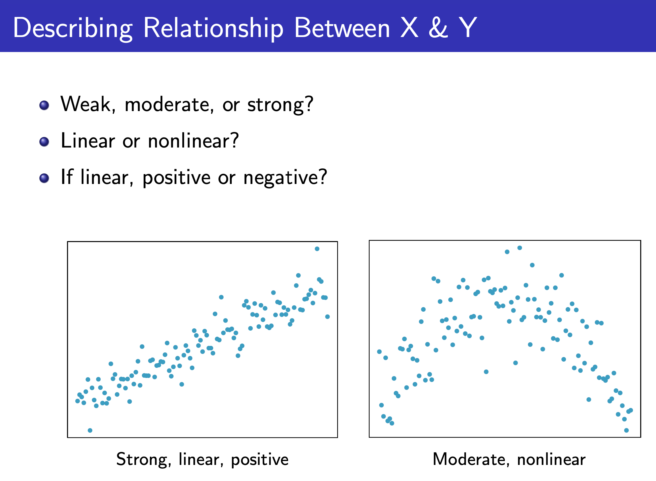
Relationship¶

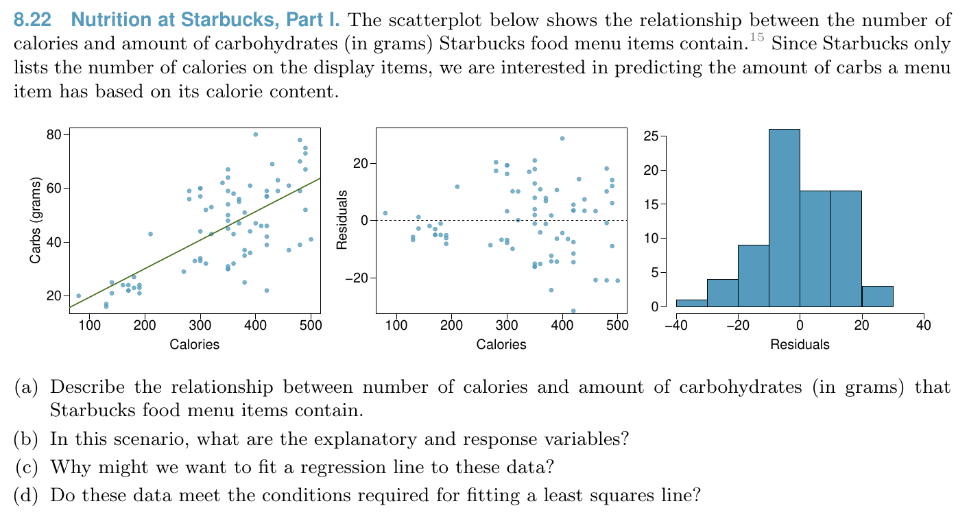
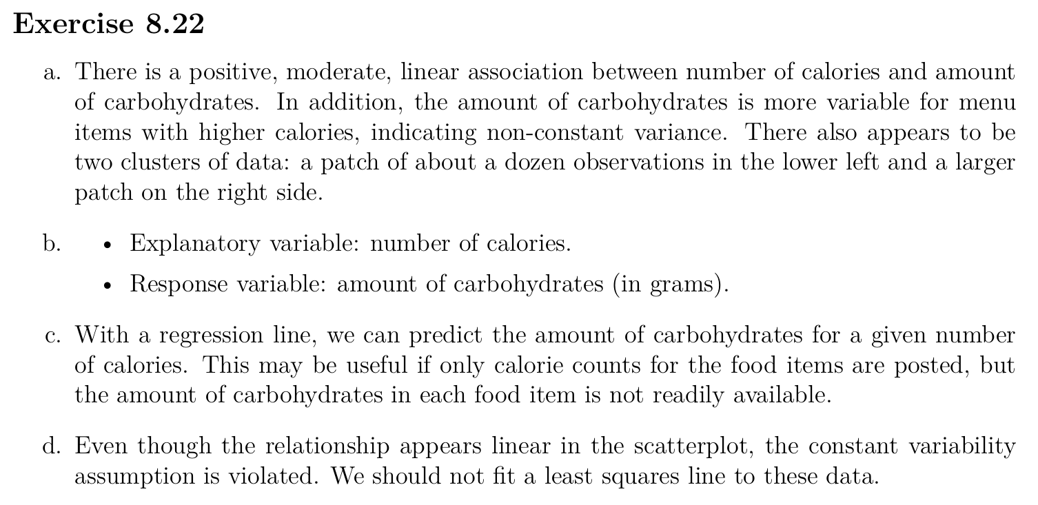
Model¶

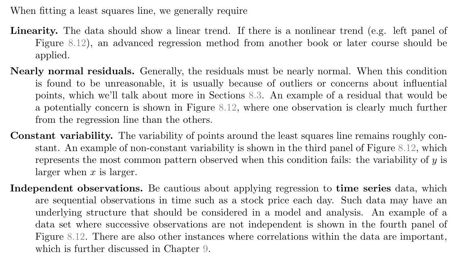
Condition of least square line