Data Structure
- inf: greatest lower bound
- sup: least upper bound
Big-Oh Notation
檢測
- \(f(x)=\dfrac{h(x)}{g(x)}\)
- \(\lim_{x\to\infty} f(x)\)
- \(\lim_{x\to\infty} \frac{f(x+1)}{f(x)}\)
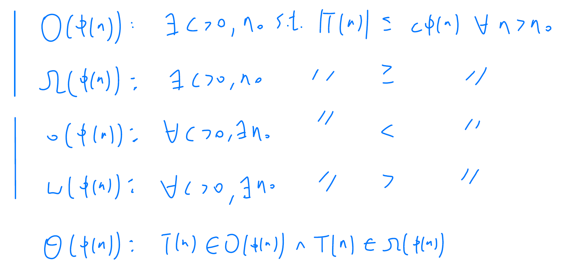
If \(\lim_{n \rightarrow \infty} \frac{|T(n)|}{\phi(n)}\) exists, then \(\(\lim_{n \rightarrow \infty} \inf_{m \geq n} \frac{|T(m)|}{\phi(m)} = \lim_{n \rightarrow \infty} \frac{|T(n)|}{\phi(n)} = \lim_{n \rightarrow \infty} \sup_{m \geq n} \frac{|T(m)|}{\phi(m)}\)\) Therefore
Properties of Big-Oh Notation
Assume all functions are positive.
- Constant factors can be ignored.
- \(kT(n) \in \Theta(T(n)), \forall k > 0\)
- Higher power grows faster
- \(n^r \in O(n^s), \forall r \leq s\)
- Fastest growing term dominates a sum
- \(f(n) \in O(g(n)) \Rightarrow f(n) + g(n) \in \Theta(g(n))\)
- Ex. \(5n^2+27n+1005 \in O(n^2)\)
- Polynomial's growth is determined by leading term.
- If \(f(n)\) is a polynomial of degree \(d\), then \(f(n) \in \Theta(n^d)\).
- Transitivity
- If \(f(n) \in O(g(n))\) and \(g(n) \in O(h(n))\), then \(f(n) \in O(h(n))\)
- Product of asymptotic upper bounds is asymptotic upper bounds for products
- If \(f_1(n) \in O(g_1(n))\) and \(f_2(n) \in O(g_2(n))\), then \(f_1(n)f_2(n) \in O(g_1(n)g_2(n))\).
- Exponential functions grow faster than powers
- \(n^k \in o(b^n), \forall b > 1\)
- Ex. \(n^{100} \in O(1.01^n)\)
- Logarithmic grows slower than powers
- \(\log_b n \in o(n^k), \forall b > 1\) and \(k > 0\).
- Ex. \(\log_2 n \in O(n^{1/3})\).
- All logarithms grow at the same rate
- \(\log_b n \in \Theta(\log_d n), \forall b,d > 1\).
- Sum of the first \(n\) \(r\)'th power grows as the \((r+1)\)'th power
- \(\sum_{k=1}^n k^r \in \Theta(n^{r+1})\), for all \(r > -1\).
- Ex. \(\sum_{k=1}^n k = \frac{n(n+1)}{2} \in \Theta(n^2)\).
The performance of an algorithm may also depend on the exact values of the data, specified by the best case, worst case, and average case performance.
題目

Analyzing an Algorithm
- Simple statement sequence
-
Time complexity is \(O(1)\) as long as \(k\) is constant
-
Simple loops
-
Time complexity is \(O(n)\)
-
Nested loops
-
Time complexity is \(O(n^2)\)
-
Loop index does't vary linearily
- h = 1,2,4,8,... until exceeding n
-
大概有 \(\log_2 n\) 項 → Time complexity is \(O(\log_2 n)\)
-
Loop index depends on outer loop index
- Inner loop executed \(1+2+...+n = \frac{n(n+1)}{2}\) times
- Time complexity \(O(n^2)\)
Let's analyze the time complexity for the following algorithms:
Example 1:
def myFunc(n):
    x = 0
    y = 0
    z = 0
    u = 0
    v = 0
    w = 0
    for i in range(n):
        for j in range(n):
            x = x + i * i
            y = y + i * j
            z = z + j * j
    for k in range(n):
        u = w + (5*k + 45)
        v = v + k*k*k
    w = u+v
    return w
Example 2:
def maxSubSum(myArray):
    maxSum = 0
    idx_start = -1
    idx_end = -1
    for i in range(0, len(myArray)):
        for j in range(i, len(myArray)):
            thisSum = 0
            for k in range(i,j+1):
                thisSum = thisSum + myArray[k]
            if thisSum > maxSum:
                maxSum = thisSum
                idx_start = i
                idx_end = j
    return maxSum,idx_start,idx_end
\(O(n^3)\)
python list actual implementation
 pop(2) 需要 O(n) at worst case
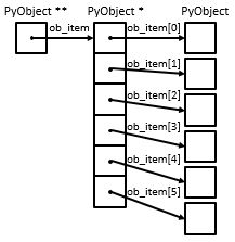
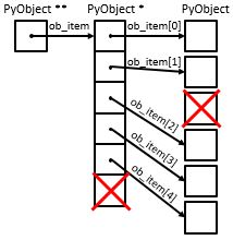
In Python’s implementation, when an item is taken from the front of the list, all the other elements in the list are shifted one position closer to the beginning. For instance, what pop(2) does is as follows:
Though it causes time for pop operation, this allows the index operation to be \(O(1)\). This is a tradeoff that the Python implementors makes based on how people most commonly use the list data structure. The implementation is optimized so that the most common operations were very fast, sometimes by sacrificing the performance of less common operations.
| Operation | Big-O Efficiency |
|---|---|
| index [] | O(1) |
| index assignment | O(1) |
| append | O(1) |
| pop() | O(1) |
| pop(i) | O(n) |
| insert(i,item) | O(n) |
| del operator | O(n) |
| iteration | O(n) |
| contains (in) | O(n) |
| get slice [x:y] | O(k) |
| del slice | O(n) |
| reverse | O(n) |
| concatenate | O(k) |
| sort | O(n log n) |
| multiply | O(nk) |
| - index[]: ** 指到 *0 → 加法到所要位置 → 指到 object |
It is should be clear that the execution time for pop(0) and pop() are O(n) and O(1), respectively.
Some sources of error occurs due to other processes running on the computer which may slow down our code. That is why loop the experiments many times to make the measurement more statistically reliable.
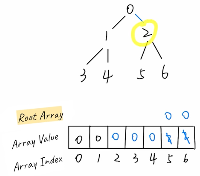
Python Built-in Dictionary Operation Time Complexity
If you were the implementor of Python, how do you implement dictionary so that the contain, get item and set item operations all have average case time complexity of \(O(1)\).?
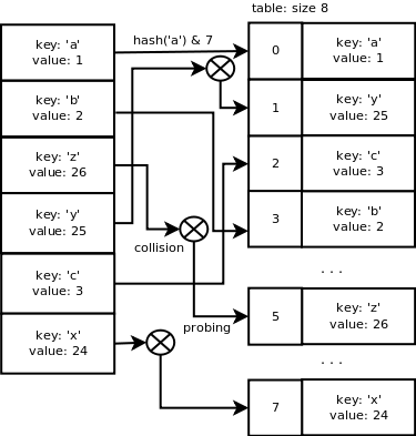
Currently, Python dictionaries are implemented as hash tables (Reference: dictobject.h). We will get into hash tables later in the course, but the following figure might give you some hints on how it works.
The average case time complexity of dictionary operations are as follows:
| Operation | Big-O Efficiency |
|---|---|
copy |
\(O(n)\) |
get item |
\(O(1)\) |
set item |
\(O(1)\) |
delete item |
\(O(1)\) |
contains (in) |
\(O(1)\) |
iteration |
\(O(n)\) |
In the following experiment we compare the performance of the contains operation between lists and dictionaries.
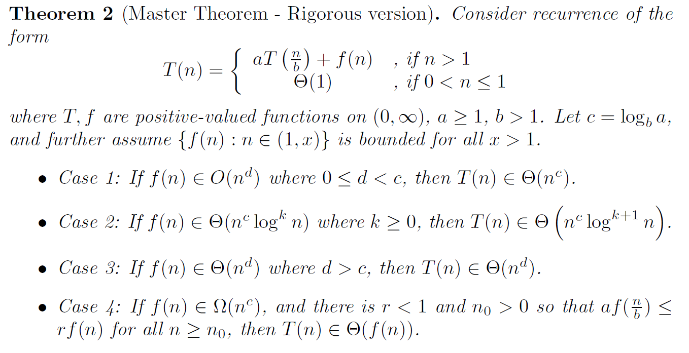
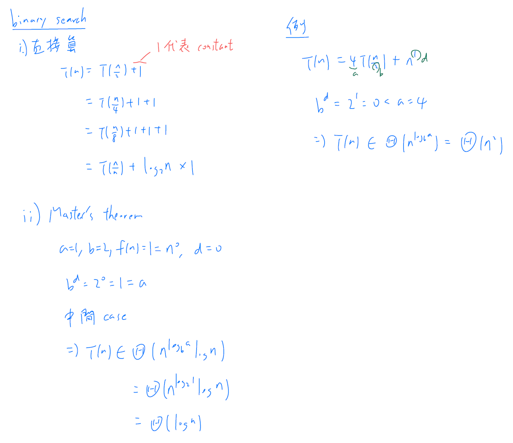
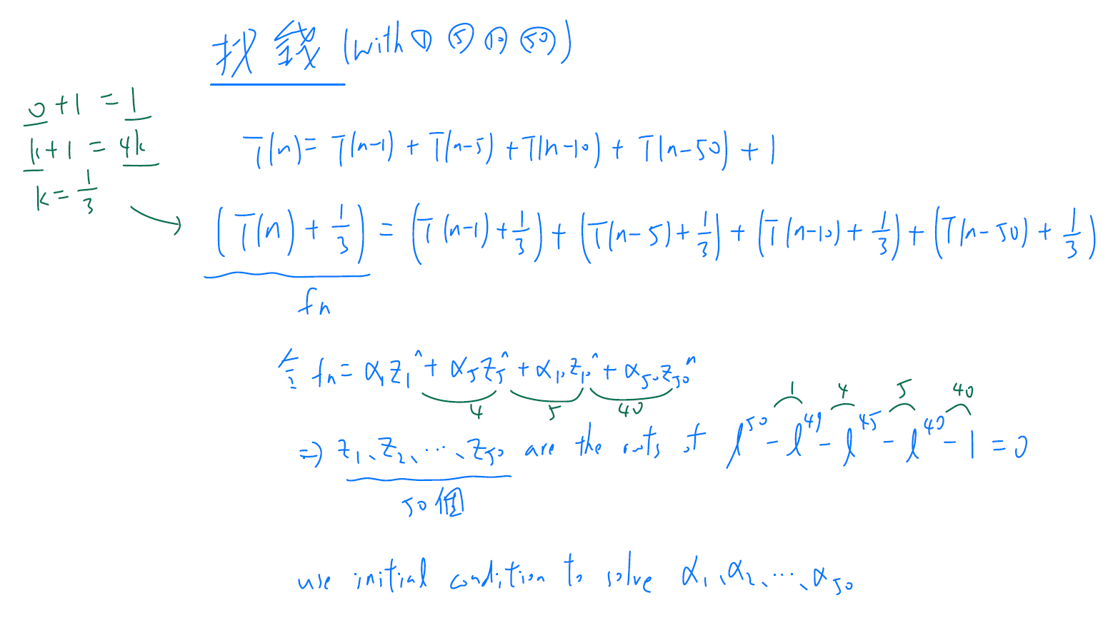
Master Theorem
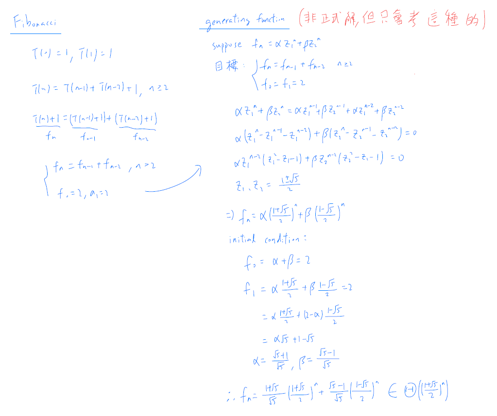
generating function
Dynamic Programming
- store the solutions
- 查表 (T(1)) instead of recursion(T(n-k))
- start from small → get big
- 用空間換取時間
Bell (W2) - https://www.geeksforgeeks.org/bell-numbers-number-of-ways-to-partition-a-set/
Tree
Binary Tree
- Binary Tree
- 每個 node 有 0-2 個分支 → binary tree
- inorder 順序正確(小→大 or 大→小) → binary search tree
- order
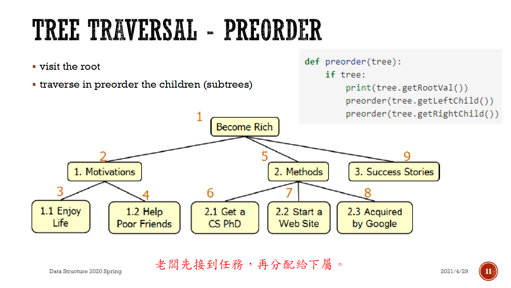
- preorder/prefix
- 接到任務的先後順序 (左支先)
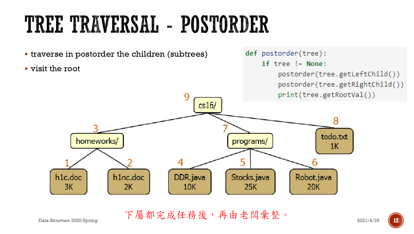
- postorder/postfix
- 完成任務的先後順序
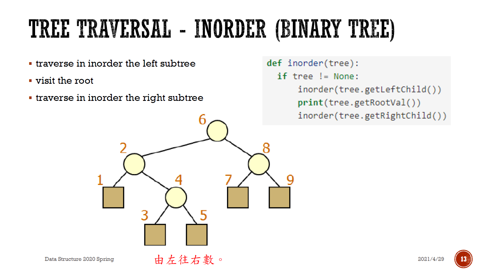
- inorder/infix
- 由左往右數
- classification
- full/proper/plane
- 每個 node 有 0 or 2 個分支
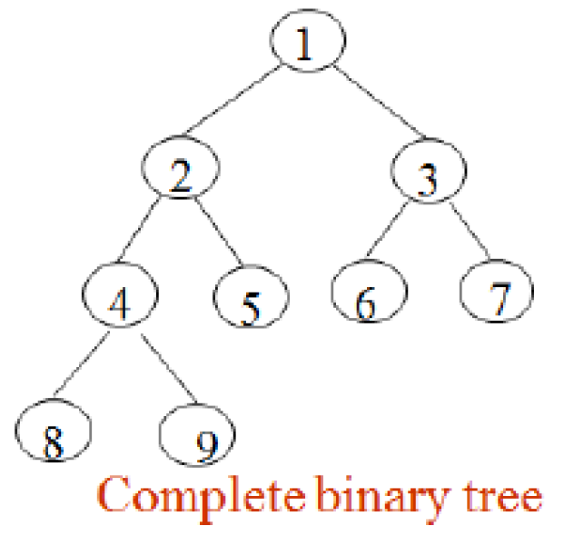
- complete
- up/left 填滿(2 分支)才能填 bottom/right
- parent of node i is node i//2, unless i=1
- left child of node i is 2i, unless 2i > n
- right child of node i is 2i+1, unless 2i+1 > n
- perfect
- symmetrical for all branches,同 level 的 node 的分支數都一樣 (balanced)
- height k → \(2^{k+1}-1\) (等比) nodes
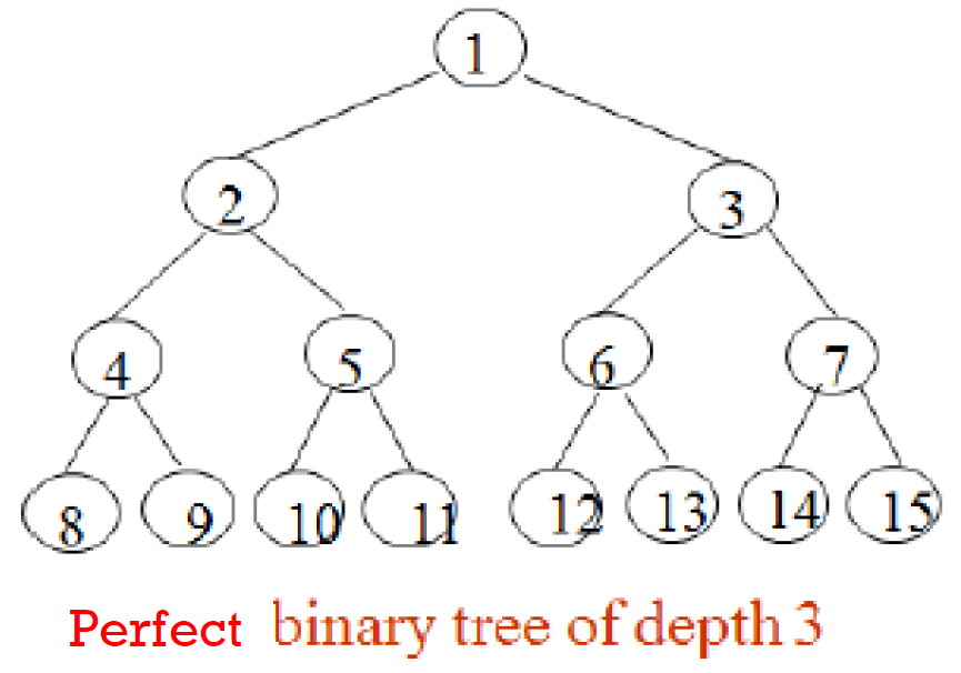
- \(k\in \Theta(logn)\) (height=k, nodes=n)
- insert O(height)
- search O(height)
- delete O(height)
- node with 1 child
- bypass 掉
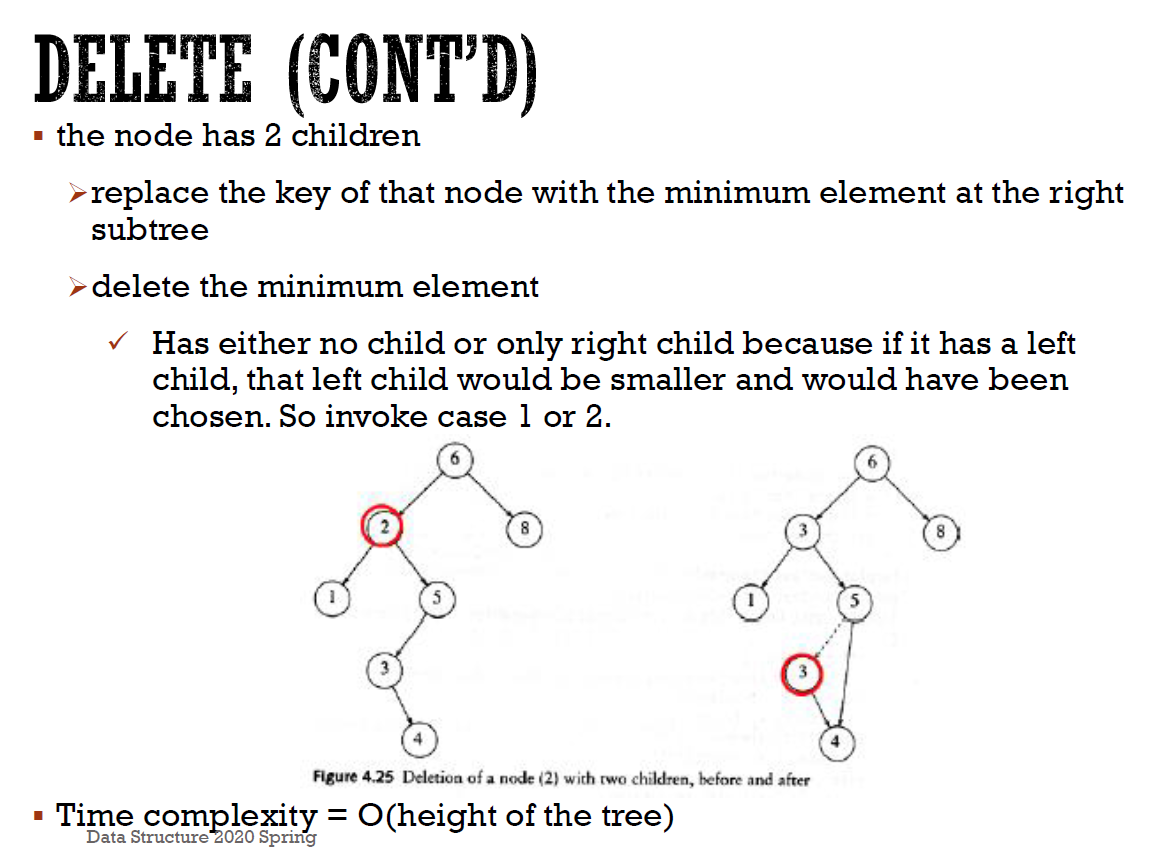
- node with 2 children
- replace with 右邊 min,並 delete/bypass 掉右邊 min
- problem
- height \(\in \Omega(logn)\) (\(O(logn)\) if perfect), worst cast O(n)
AVL Tree
- height of left & right node 之差 <= 1 的 binary search tree
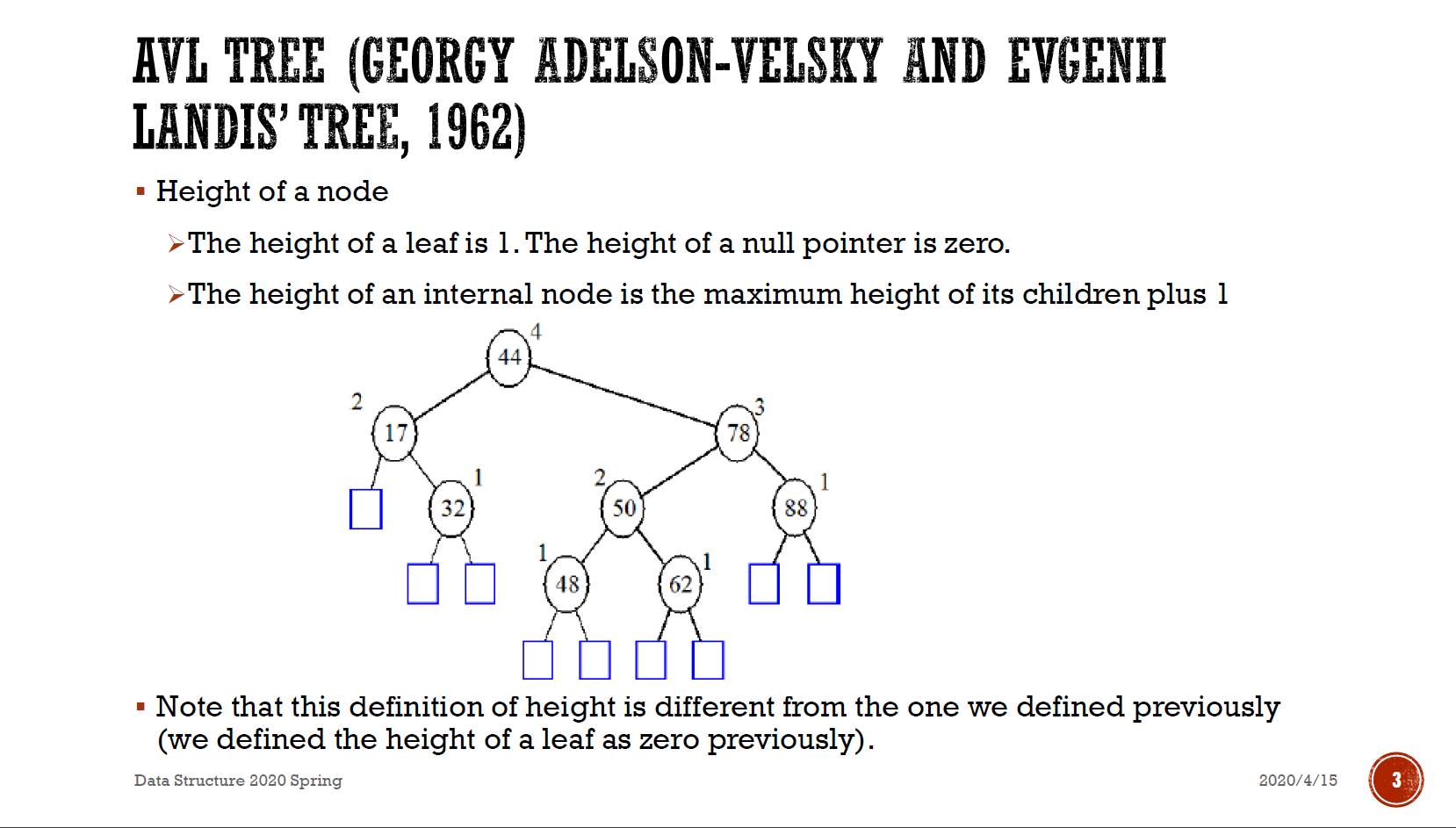
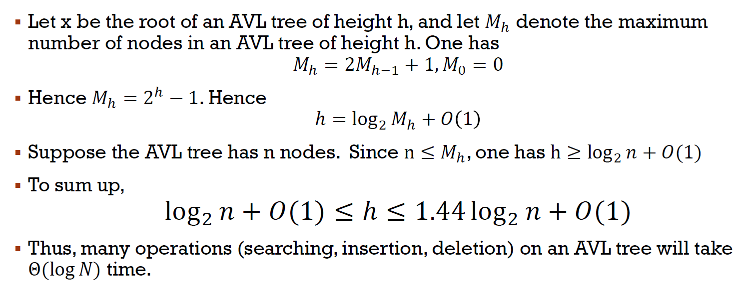
- height \(\in \Theta(logN)\)
- upper bound (兩邊高度差一, smallest)
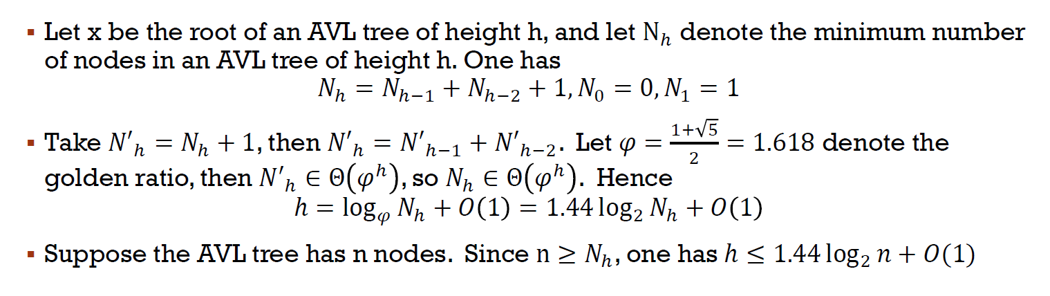
- lower bound (兩邊等高, biggest)
- rotation
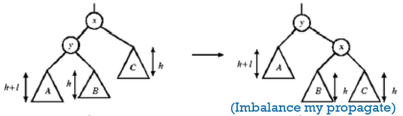
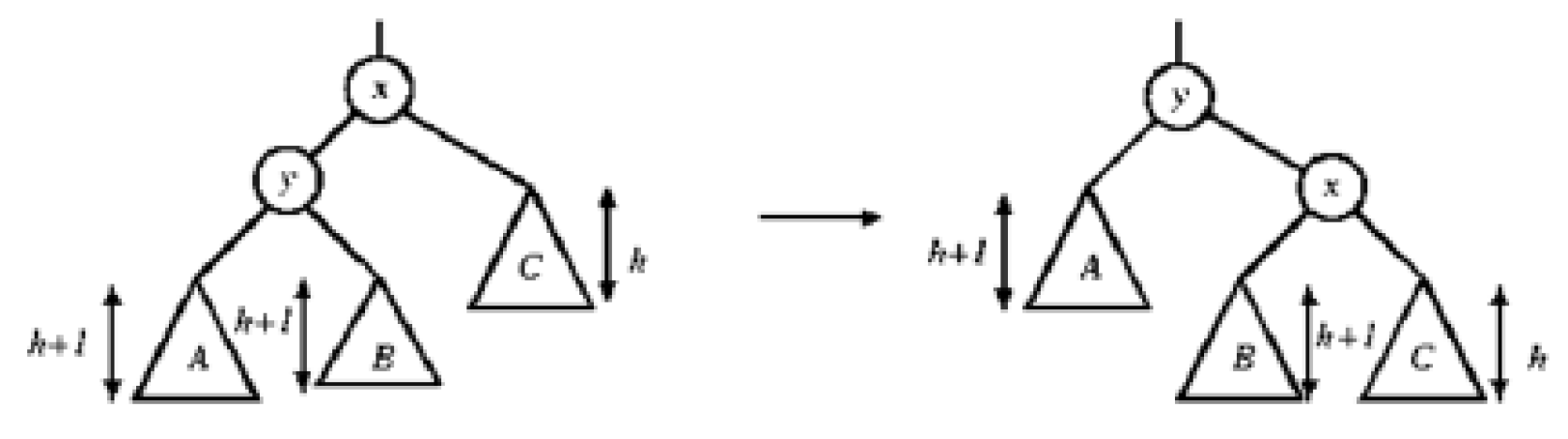
- single rotation
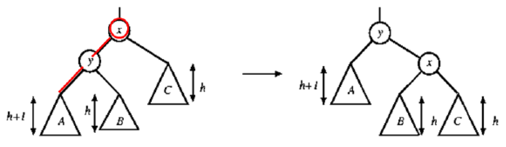
- 原是一個 AVL Tree,x = h+2
- insert C → x = h+1 but unbalanced
- 弄成右圖 → y = h+2
- so 對其他地方而言,不變 as 前後都是 h+2,so 整株樹仍是 AVL Tree
- 檢查:
- A < y
- A < y < B
- y < B < x
- x < C
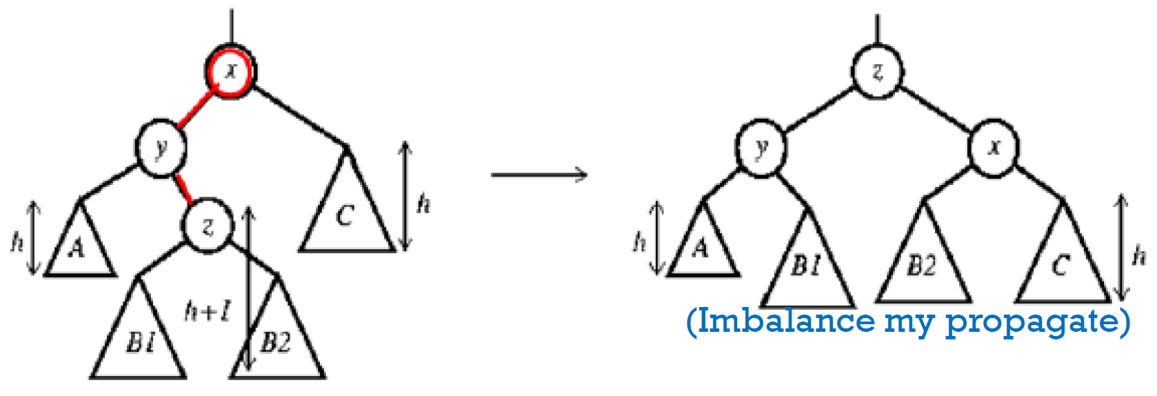
- double rotation
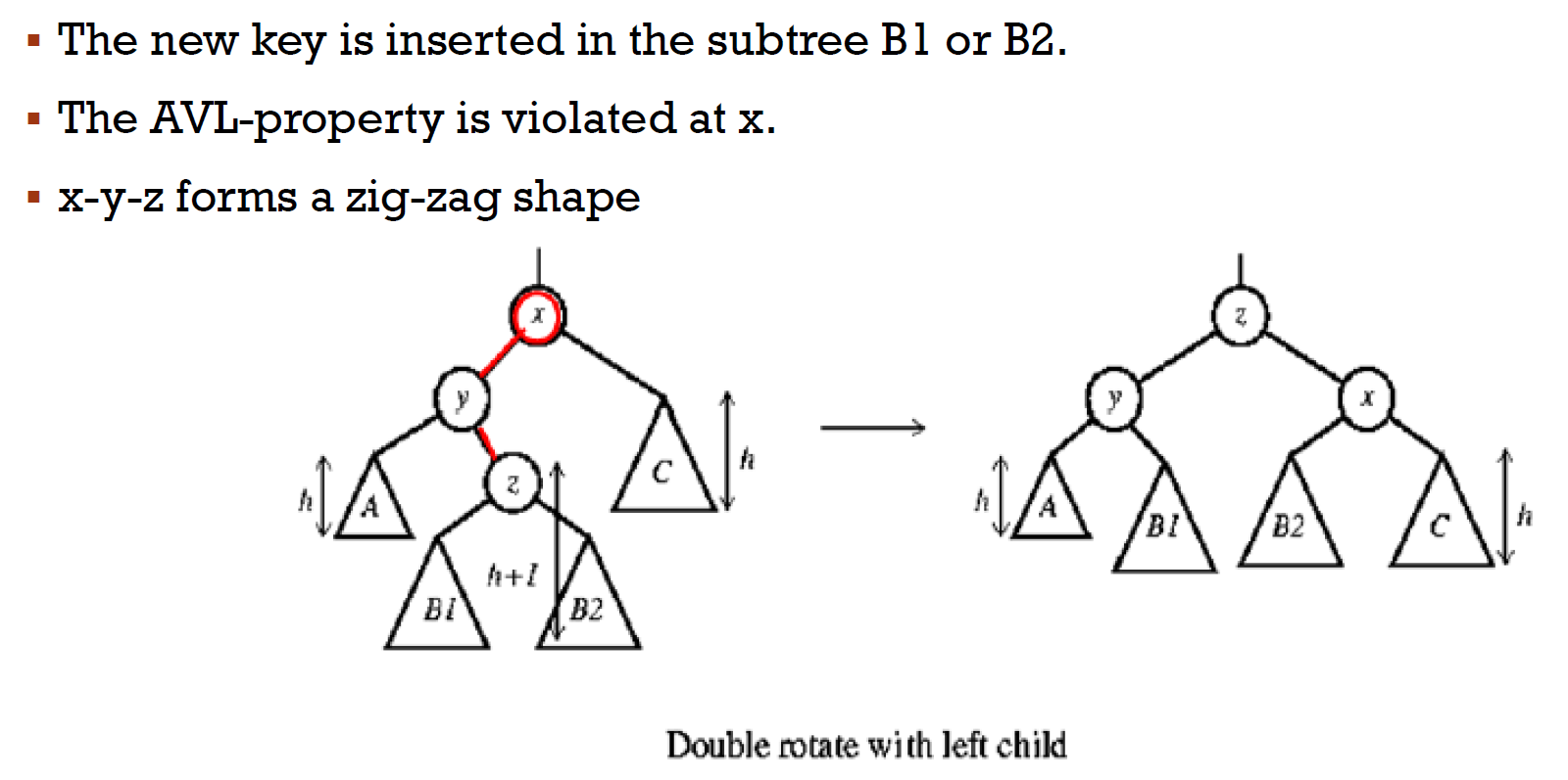
- insert B1 B2 後,(由下往上)到 x 才 violate,so B1/B2 = h/h-1
- 檢查
- 左右圖看進去的 height 相同 → 整株都符合 AVL property
- 各個 node
- 重的(比較高的)在內側 → double rotation
- otherwise → single rotation
- insertion/deletion
- 傳統 binary search tree 作法
- 往上找,看有無違反 AVL property; if yes → rotation
- insertion 最多只要 rotate 一次就全 ok
- deletion 需要找到 root 才能完全確定,可能 rotate 很多次
- 上方的 node: h+3 → h+2
- 上方的 node: 不變
- pros
- search \(\in O(logN)\)
- insertion & deletion \(\in O(logN)\)
- height balancing (rotation) 只是加 constant
- cons
- 麻煩
- height 還有另外存
- asymptotically faster but rebalancing costs time
- 其他的資料結構也許需要 O(N) 做動作,但會讓後續許多其他動作比較快 → faster in the long run
- e.g. Splay tree
Splay Tree
- 性質
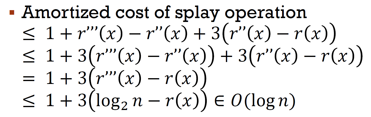
- per operation \(\in O(N)\)
- amortized time \(\in O(logN)\)
- good locality
- 常用的會在上面
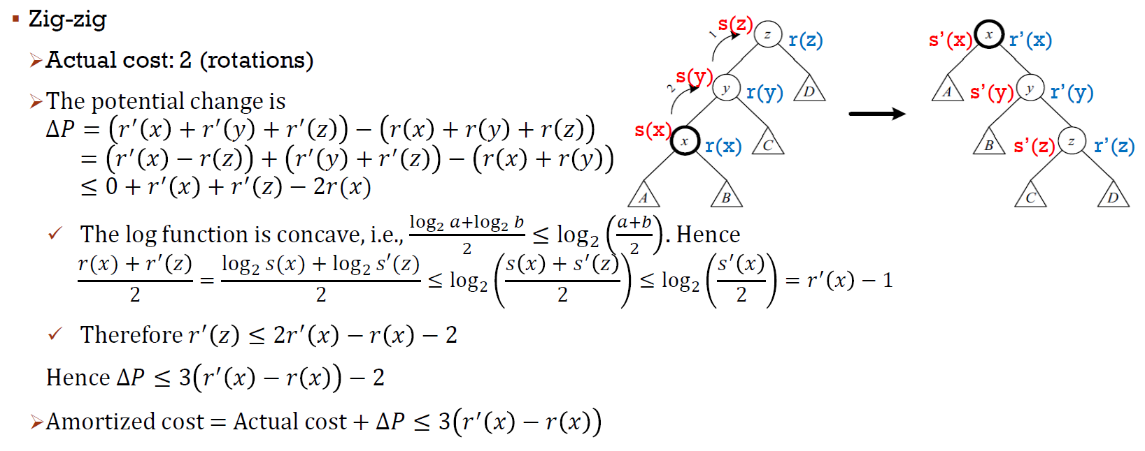
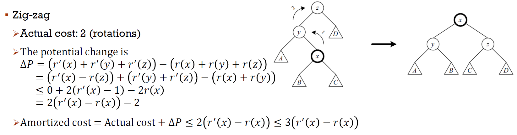
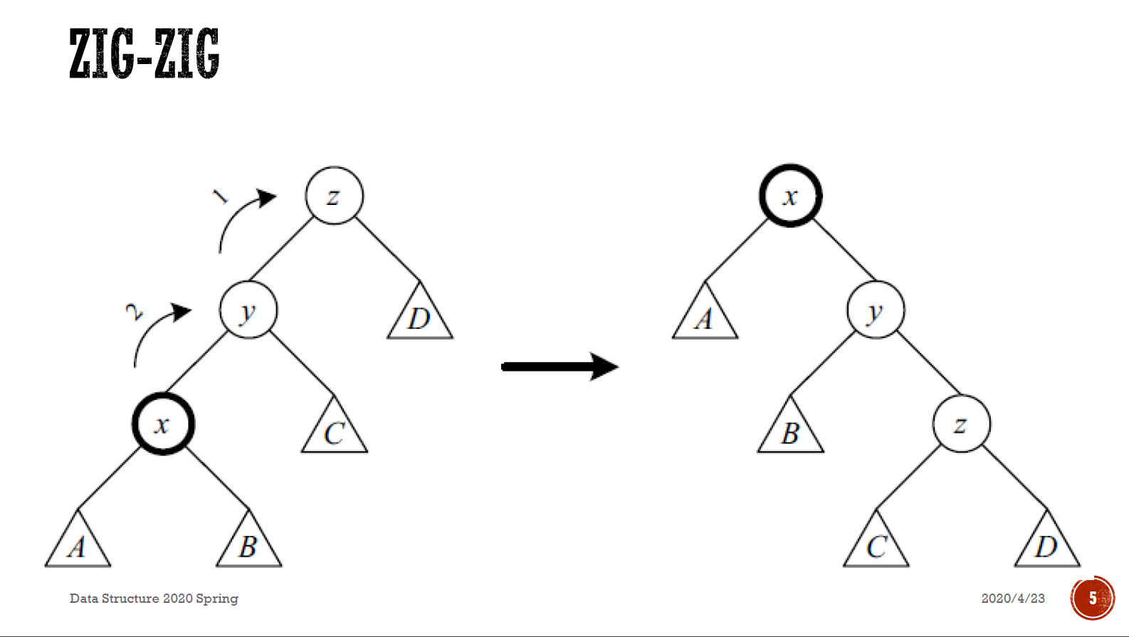
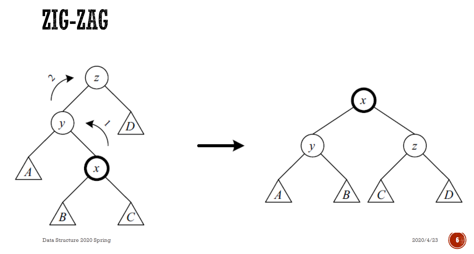
- splay
- x 在外側 → zig-zig
- x 在內側 → zig-zag
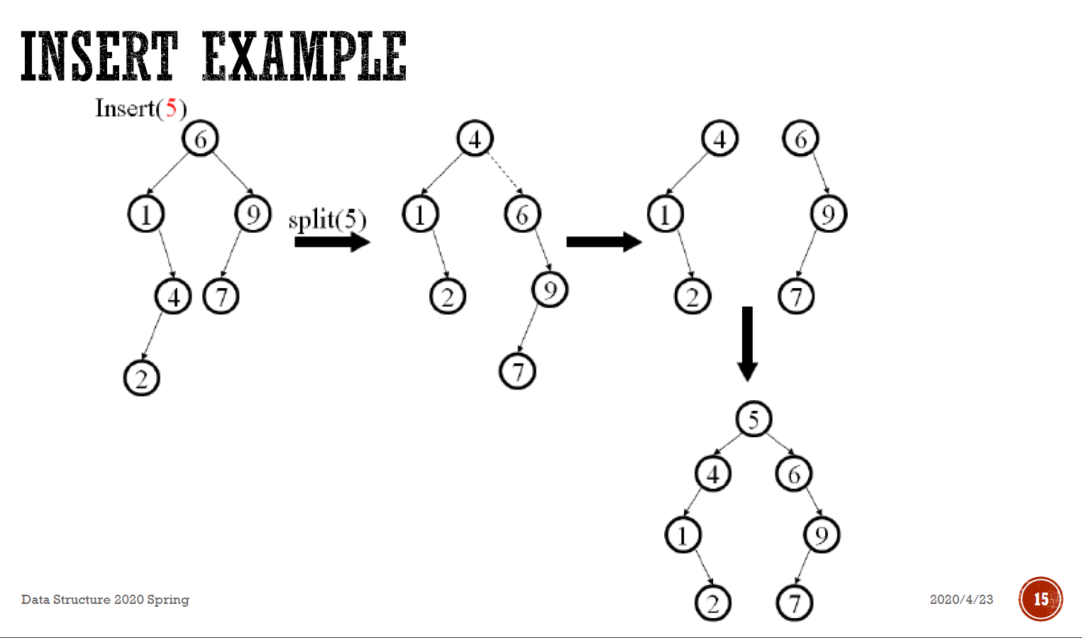
- insertion
- 把找到的那個 node splay 上去
- 就是最後一個在的 node
- split
- 插進去
- e.g.
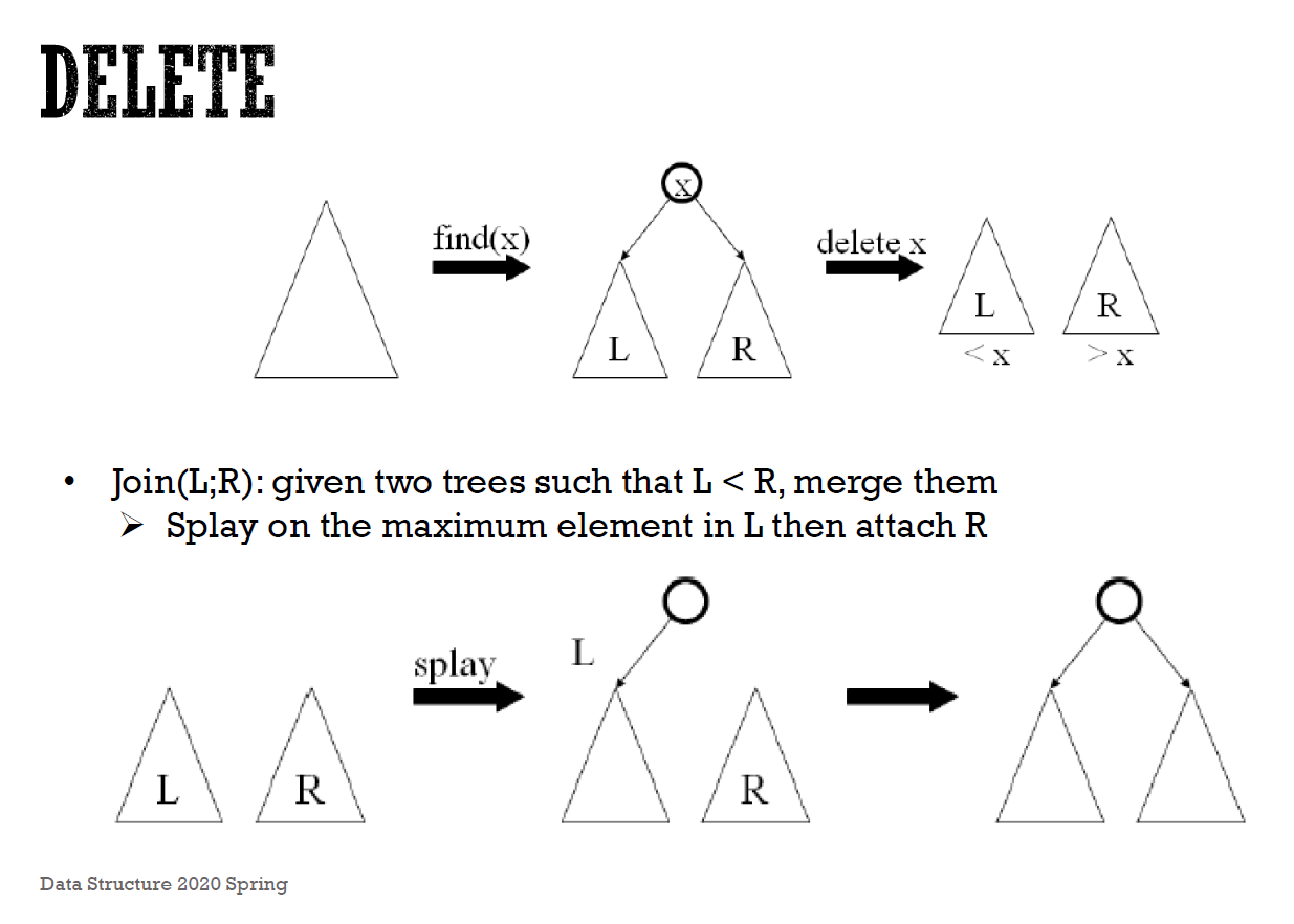
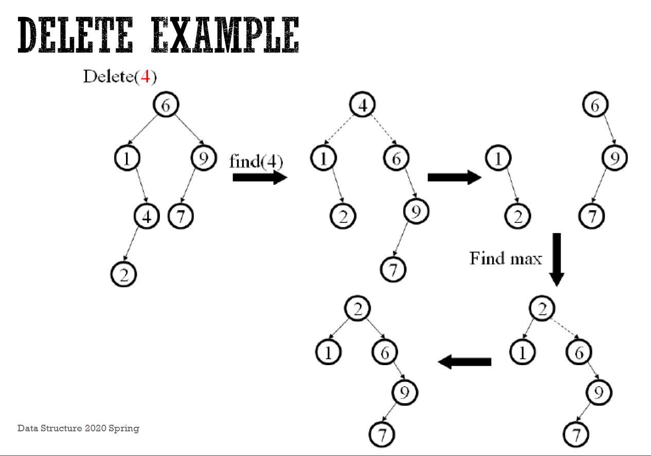
- deletion
- 把目標 node splay 上去
- delete 目標 node,變成兩個分開的 subtree
- 把 left subtree 的 max node splay 上去
- 接上 right subtree
- e.g.
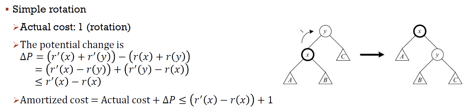
- amortized cost
- zig-zig
- zig-zag
- simple rotation
- locality
- 如果都只對幾個 node 操作 → 很快
- top-down splay
- 深度為偶數 → 結果跟 bottom-up 一樣
- 深度為奇數 → 結果可能跟 bottom-up 不一樣
Multi-Way Search Trees
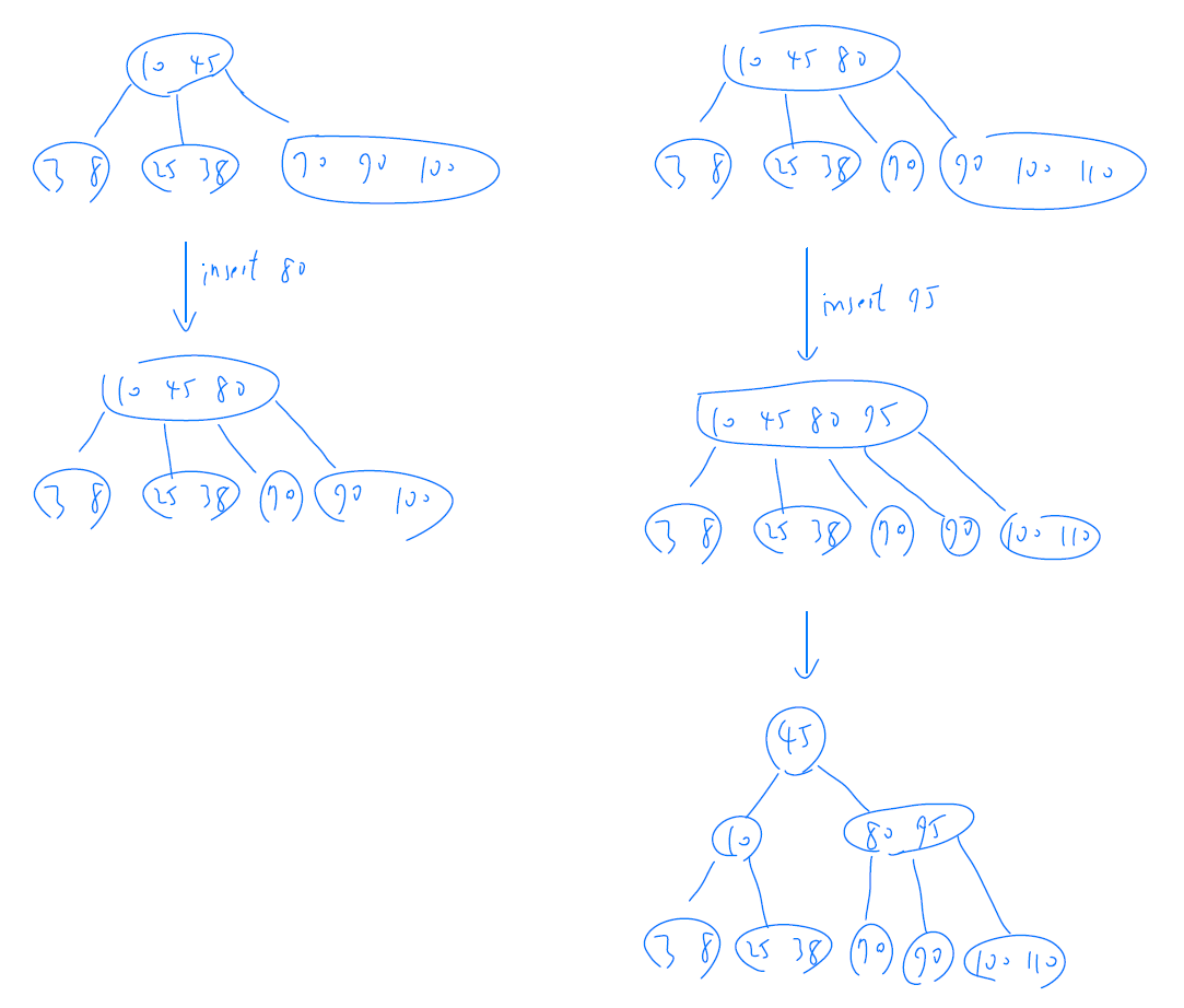
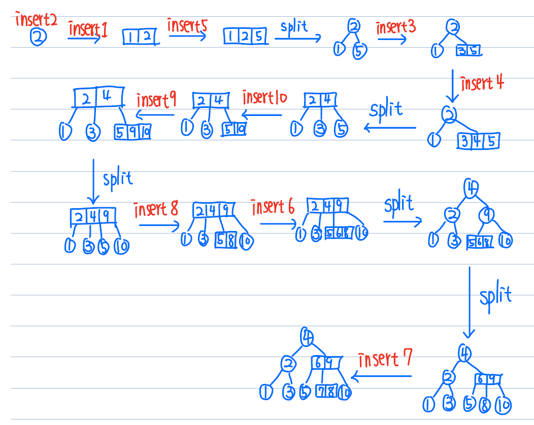
2-3-4 Tree
- all leaf on same level
- each node has 1/2/3 items
- k items → k+1 children
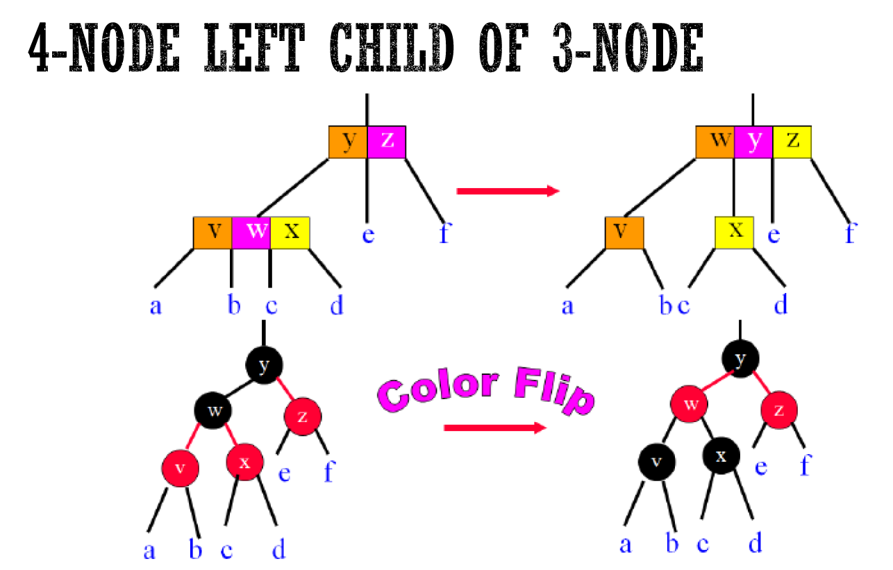
- insertion
- insert 到 leaf node
- look before you leap
- 經過的每個 4 node 都要 split
- insert 的目的地是 4 node 時,先 split 再 insert
- https://www.educative.io/page/5689413791121408/80001
- deletion
- bottom-up
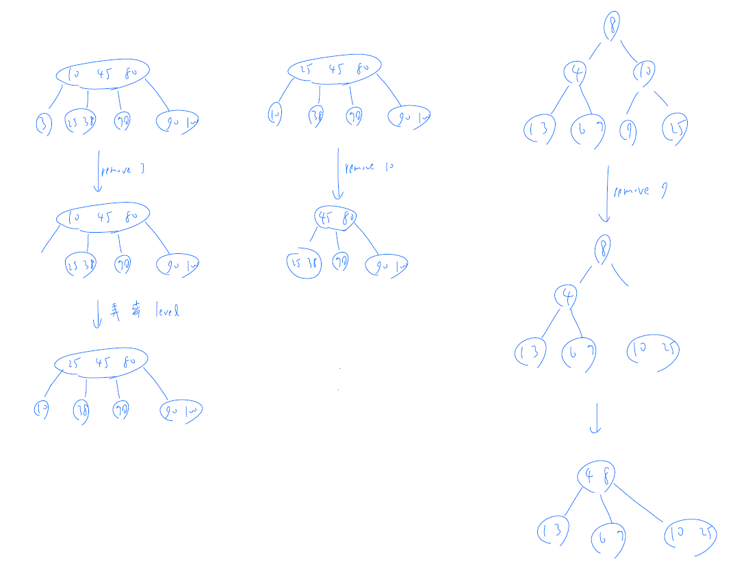
- top-down
- look before you leap
- 經過的每個 2 node 都要 split
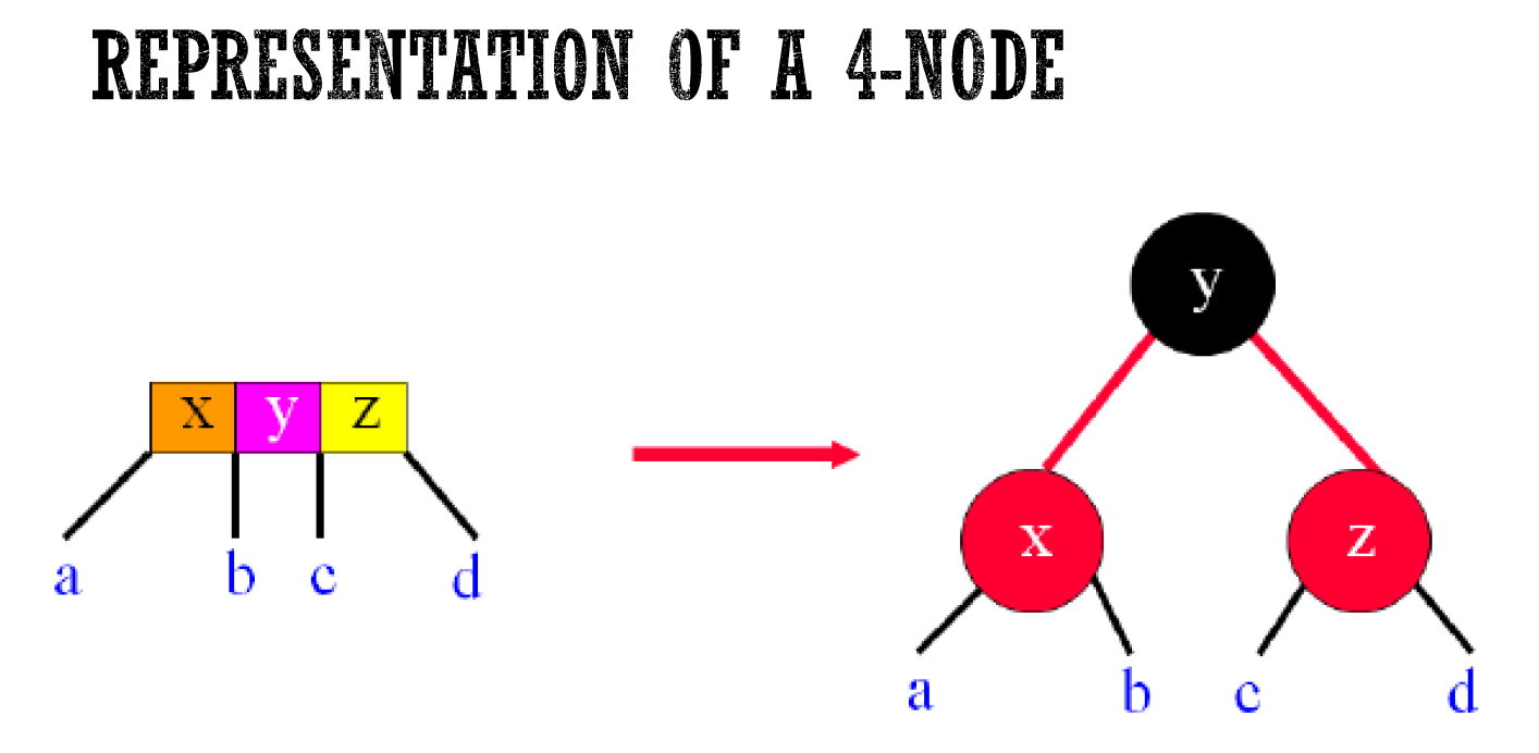
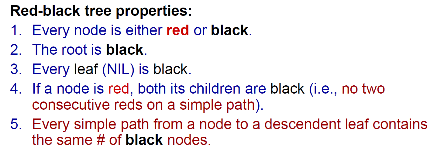
Red-Black Tree
- Red-Black Tree
- represent 2-3-4 tree as binary tree
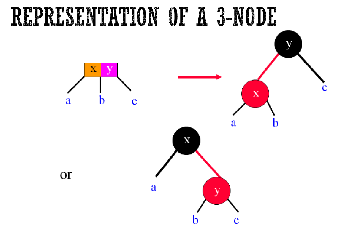
- 兩種表示法
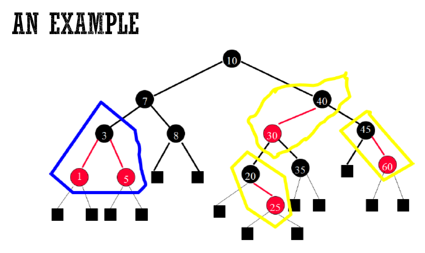
- properties
- root 是 black
- 注意 ==leaf 是指 NIL==,永遠是黑色
- 不會連續兩個 red
- 每個 path 黑 node 數都一樣
- 2-3-4 leaf nodes 都同 level
- max height \(2log(n+1)\)
- https://www.codesdope.com/course/data-structures-red-black-trees/
- https://doctrina.org/maximum-height-of-red-black-tree.html
- W4-2
- operation:先做 2-3-4 再轉成 Red-Black
AA Tree
- interactive visualization
- Red-Black Tree but left-child can't be red
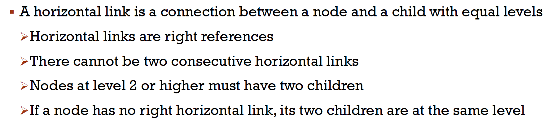
- level
- leaf = 1
- red = parent's level
- black = parent's level - 1
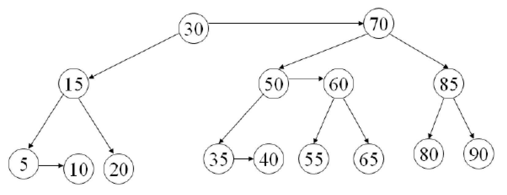
- 水平:同 level (必指到 red)
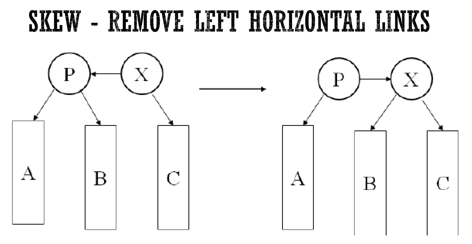
- operations
- skew:
- remove 1 left horizontal
- add 1 right horizontal
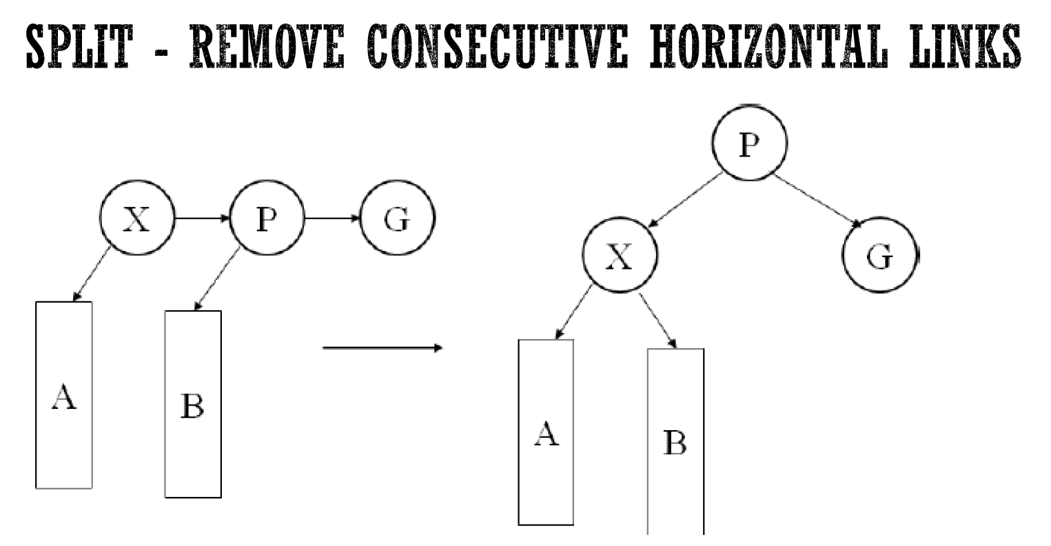
- split
- remove consecutive right horizontal
- 把中間堤上去
- 不會考 deletion
hash
- hash function
- \(h(k)=k\%m\)
- 避免是 m≒2^n bc 二進位數/2^n 就是後 n 個 digit 而已
- 設 m = 質數
- 若 k = m 的因數的倍數,則只會用到某幾格
- e.g. key%3=0,m=18 → 只會用到 6 格
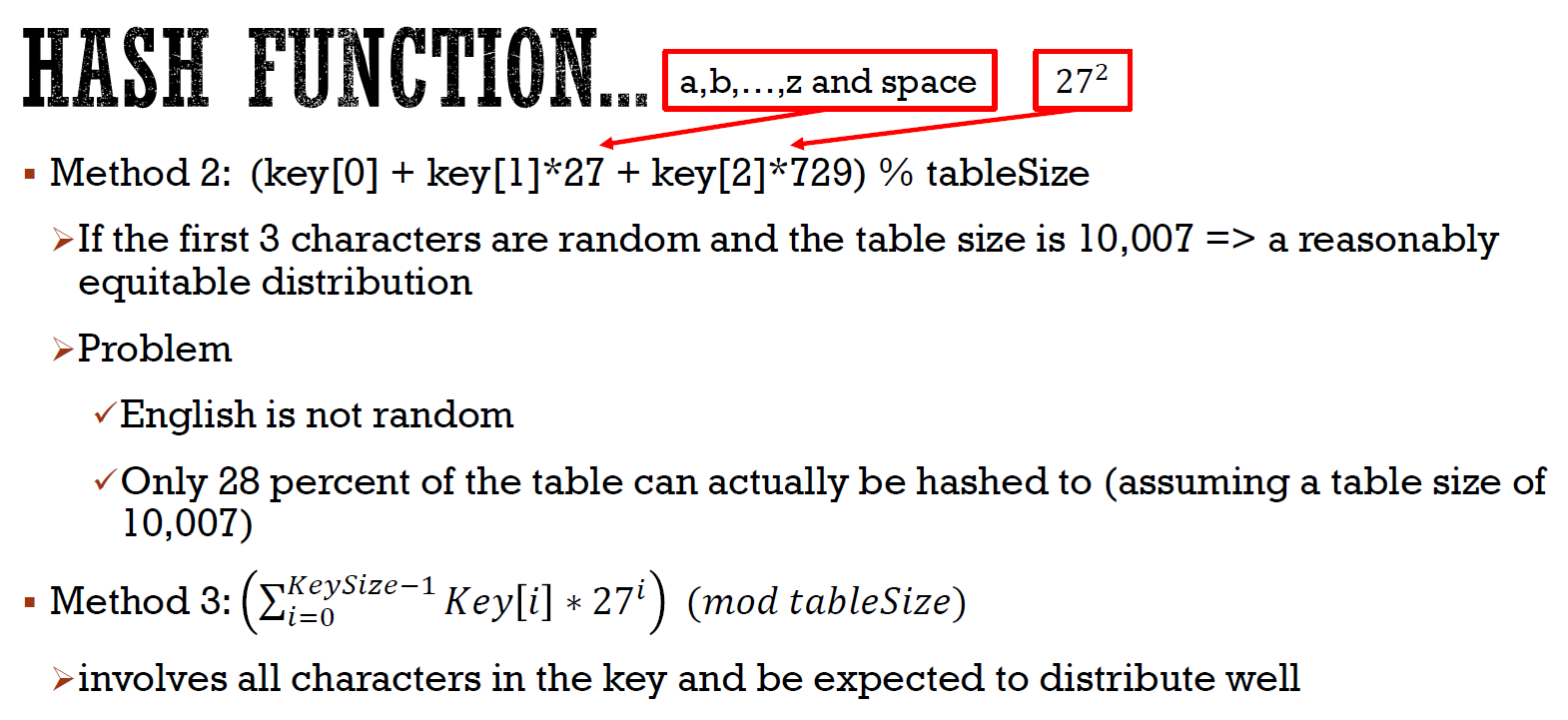
- 若 key 是 string
- sum of ASCII
- len = 8 → 只會用到 127x8 個 slot
- separate chaining
- 可每個 slot 存 linked list
- collision → 加到後面
- insertion O(1)
- 加到前面
- deletion/search O(長度)
- open addressing
- collision → relocate
- \(h_i(k)=(h(k)+f(i))mod\space m\)
- linear probing
- \(h_i(k)=(k+i)mod\space 10\)
- collision → 跳一格
- 會形成 cluster → 耗時
- quadratic probing
- \(h_i(k)=(k+i^2)mod\space 10\)
- double hashing
- \(f(i)=i\cdot h_2(k)\)
- \(h_2(k)=R-(k\space mod\space R)\)
- bc \(h_2(k)=0\) → 跳零格 → 沒屁用
- 就是 collision 時每次跳的格數
- \(h_i(k)=(k+i(R-(k\space mod\space R)))mod\space m\)
- e.g. \(h_i(k)=(k+i(7-(k\space mod\space7)))mod\space 10\)
- \(gcd(m,h_2(k))=1\)
- e.g. R, m = prime AND R < m
- deletion
- delete 後要留個墓碑標示先前有人,表示之後 delete 到這空格時要繼續 hash
- insert 到墓碑時,就直接佔用
heap (priority queue)
bineary heap
- complete binary tree
- all levels are filled except leaf
- 先 fill 左邊
- \(h\in O(logn)\)
- MinHeap: parent key <= child key
- MaxHeap: parent ket >= child key
- insertion
- 先 insert 到最後一項 (最右 leaf 之右),再根據大小 percolate up
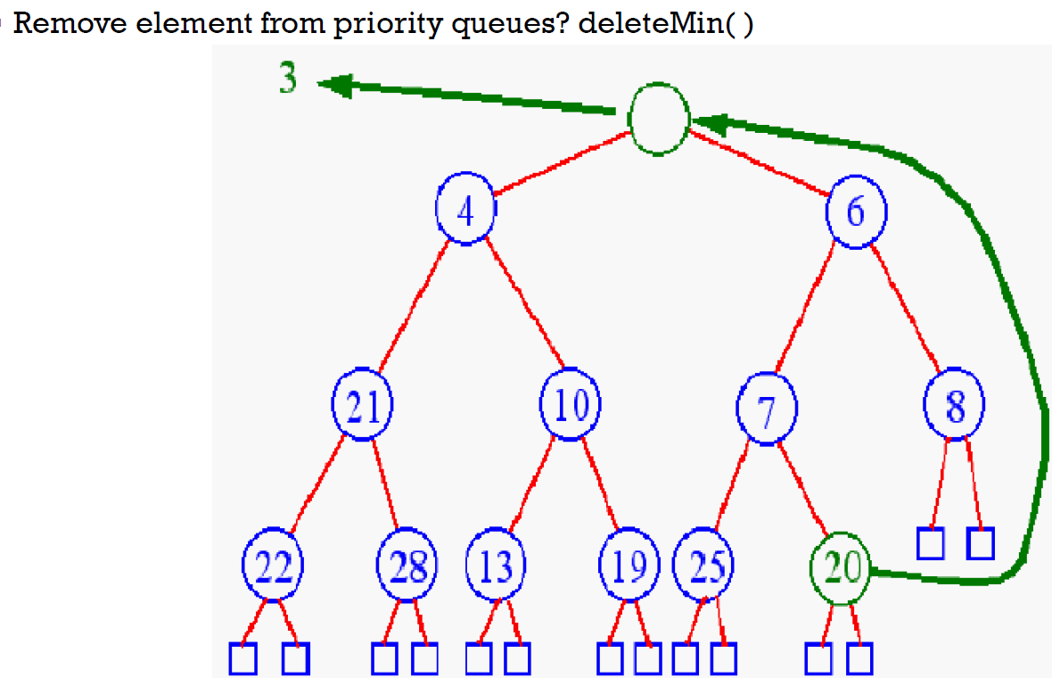
- deletion
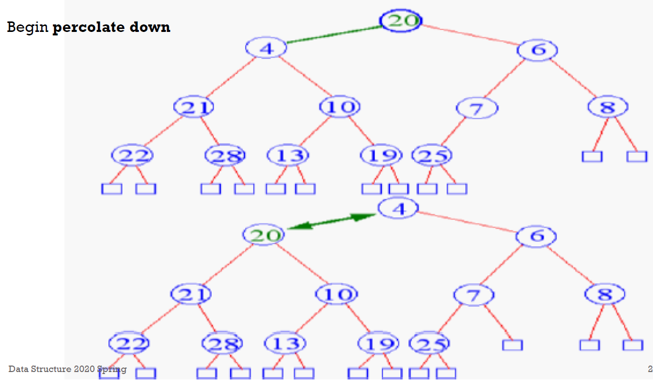
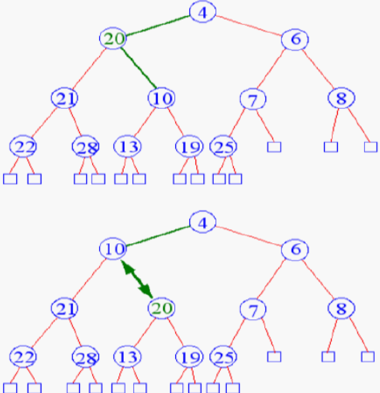
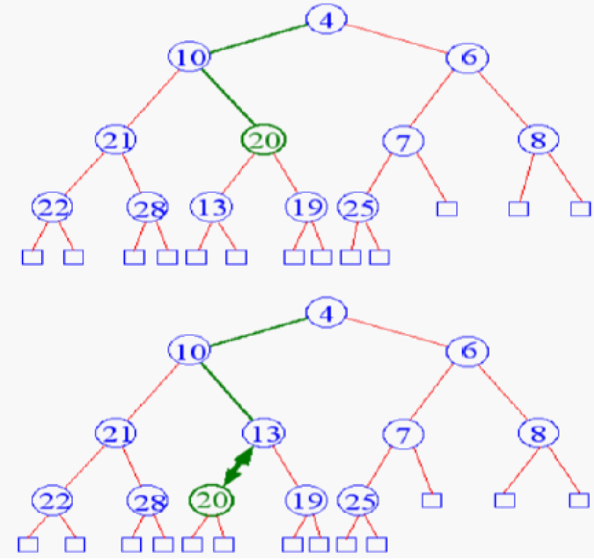
- delete root (min) → 把 bottom level 最右的 node 放到 root → percolate down
- 跟較小的且最小的 children 互換
- s.t. children 被換上去後也會小於另一個 children
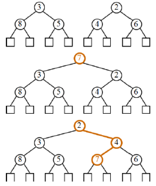
- merge
- 先放到 root 再 percolate down
- bottom-up construction
- o(n)
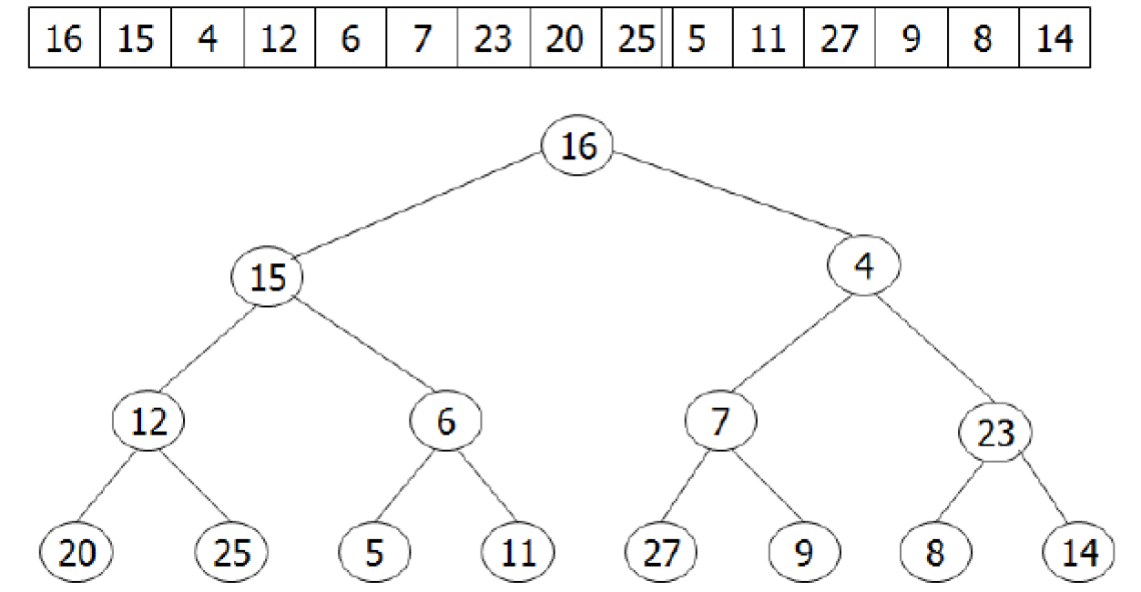
- array representation
- index start from 0
- left child = 2i+1
- right child = 2i+2
- i = odd → left child
- i = even → right child
binomial heap
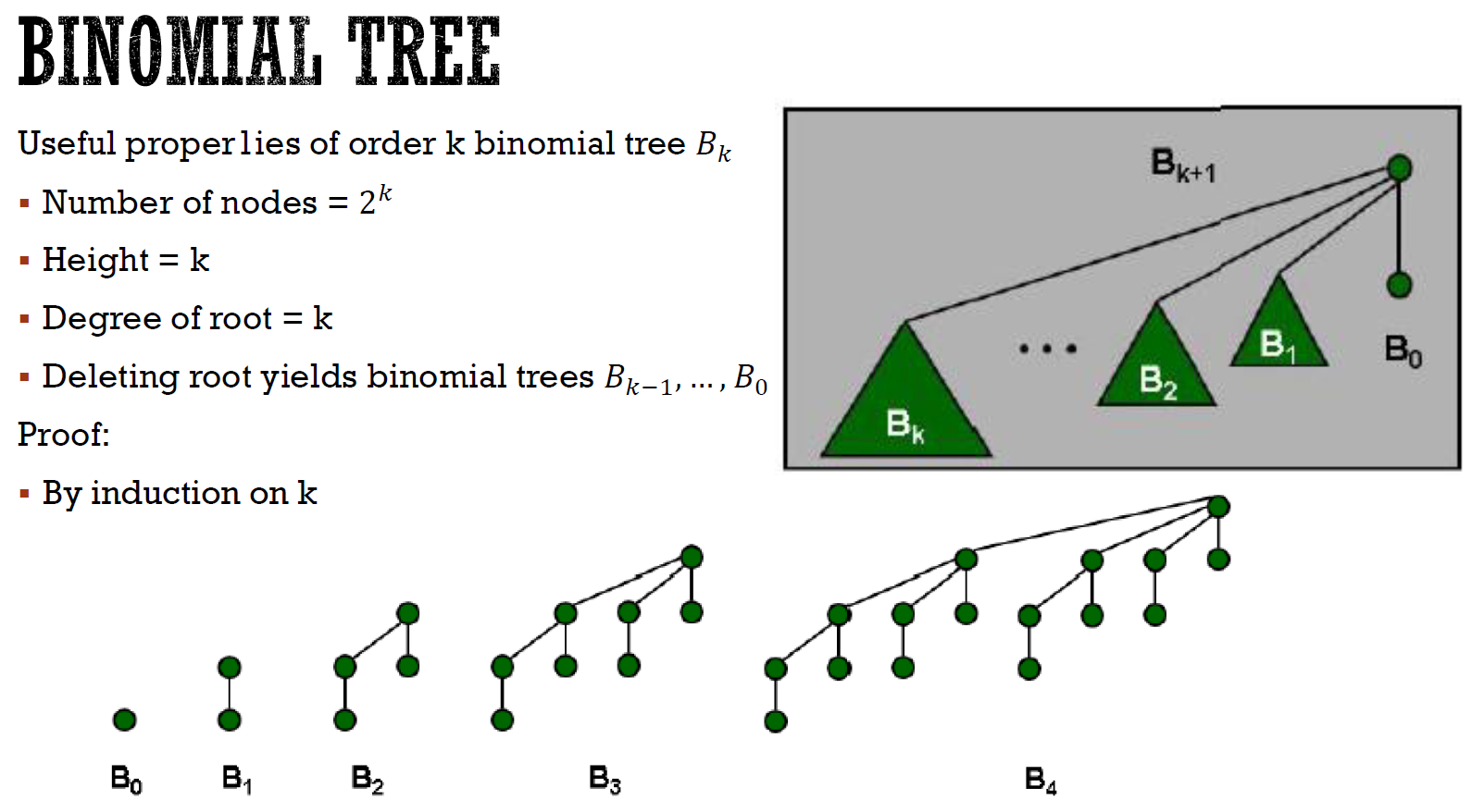
- height = k
- \(2^k\) nodes
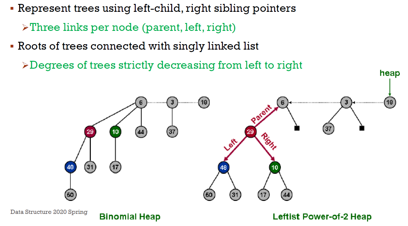
- roots 是 singly linked list
- 砍掉 root → k 個 binomial tree
- 每棵都是 min 形式 (大的在下,小的在上)
- n 個 nodes 只會有一種結構
- 每棵樹的 order 都不一樣
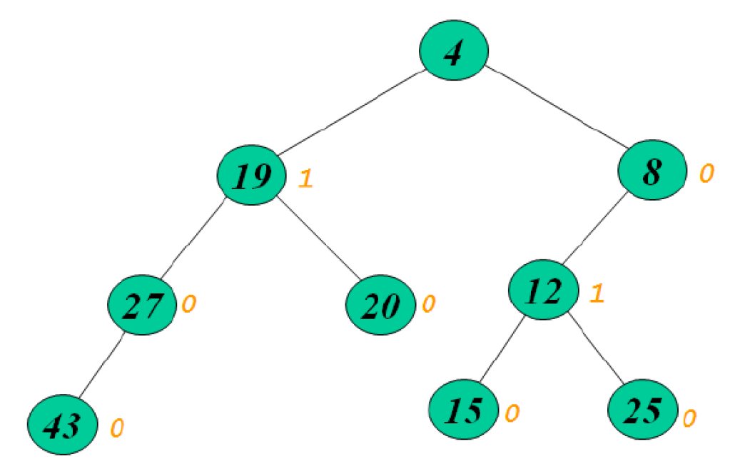
- n 個 nodes → 一種二進位表示法
- \(19 = (10011)_2\) → \(B_4\) + \(B_2\) + \(B_1\)
- \(k \leq \lfloor{log(n)}\rfloor\)
- \(2^k\leq n<2^{k+1}\) → \(log_2(n)-1 < k\leq log_2(n)\)
- at most \(k+1\) (\(B_0\)~\(B_k\)) $\leq \lfloor{log(n)}\rfloor+1 $ 個 tree
- union
- 大的接到小的 root 下
- 二進位加法
- order 相同 → merge → repeat
- 每個 order 只能有一棵樹
- delete min
- 砍掉最小 root → union rest
- \(\in O(log(n))\)
- decrease key
- key 變小 → 重新 order (like percolate up for minheap) to match heap order (parent < child)
- \(\in O(logn)\)
- deletion
- 把目標 key decrease 成 -inf → delete min → union
- \(\in O(logn)\)
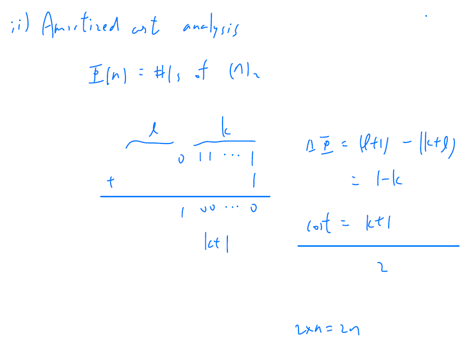
- insertion
- worst case \((111...11)_2+1\) → \(log_2n\) time
- 等同於跟 union(x,H)
- construction
- sequence of inserts
- \(\in O(n)\)
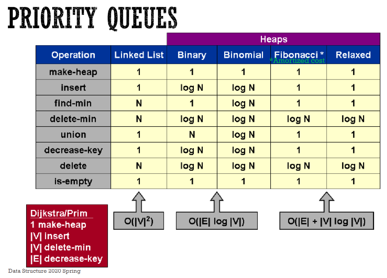
comparison
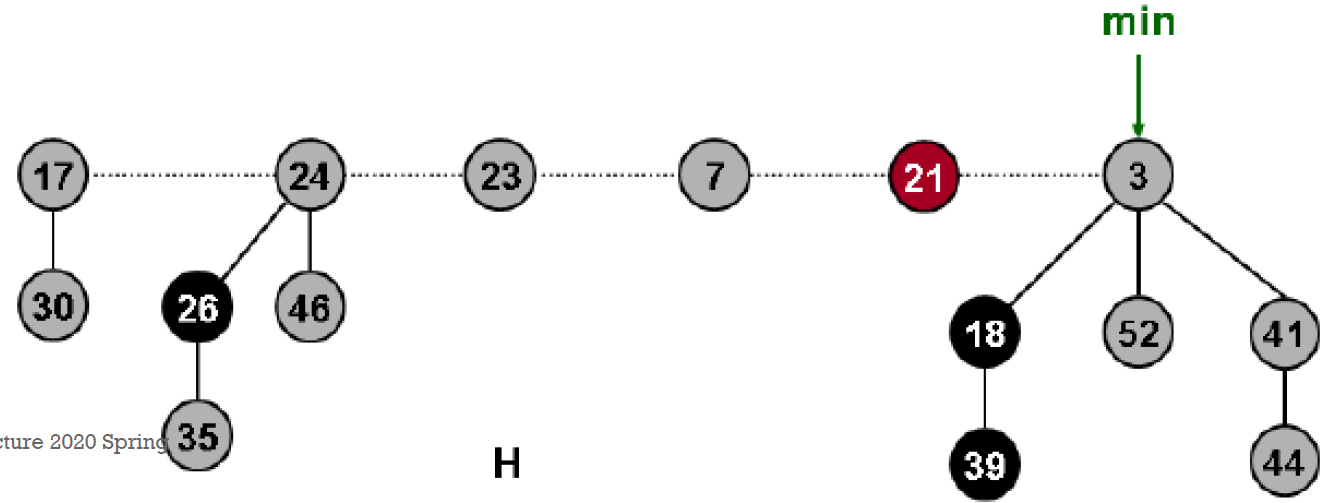
Fibonocci heap
- roots of trees → circular linked list
- degree
- root 有幾個小孩
- t(H):幾棵樹
- m(H):幾棵 marked 的樹
- \(\phi(H)=t(H)+2m(H)\) potential function
- insertion
- 放在 min 的左邊
- amortized cost O(1)
- actual cost O(1)
- potential += 1
- t(H) += 1
- m(H) += 0
- union
- 剪開 → 連起來 → update min (among circular linked list roots)
- amortized cost O(1)
- actual cost O(1)
- potential += 0
- t(H) += 0
- m(H) += 0
- delete min
- 步驟
- delete min O(1)
- 把原 min 的 children 接上 root list O(D(n)))
- consolitdate O(t(H)+D(n)) (bc worst case t(H)+D(n) 棵樹)
- 檢查每個 root 的 degree
- 若有一樣的,則把較大的 root 接在較小的下面
- amortized cost O(D(n))
- actual cost O(D(n)+t(H))
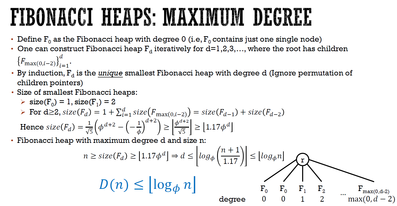
- D(n) = max degree of Fibonocci heap with n nodes
- t(H) = 原 tree 數
- potential += O(D(n)-t(H))
- t(H) += (D(n)+1-t(H))
- 原 t(H)
- 做完後 max D(n) + 1
- D(n-1) <= D(n)
- n-1 個 node 的 max degree <= n 個的
- 每棵 degree 不重複 → 0, 1, 2, ..., D(n) → max D(n)+1 棵
- m(H) += 0
- if 只做 insertion, delete-min & union → only contains binomial tree
- so \(D(n)\leq\lfloor log_2n\rfloor\)
- decrease key (x)
- parent of x = p[x]
- case 0:仍為 min-heap → 就這樣
- case 1:violate min-heap property and p[x] unmarked
- x 跟 p[x] 斷開
- mark p[x]
- 接上 root list
- unmark x
- update min
- case 2:violate min-heap property and parent marked
- x 跟 p[x] 斷開
- x 接上 root list
- 從 x 原鍊上溯
- while parent is marked, cut off link with parents, 接上 root list,再上溯
- elif unmarked → mark it,並終止上溯
- amortized cost O(1)
- c = 幾個獨立出來
- actual cost O(c)
- potential += 4-c
- t(H) += c
- m(H) += 1-(c-1) = 2-c
- c+2(-c+2) = 4-c
- deletion
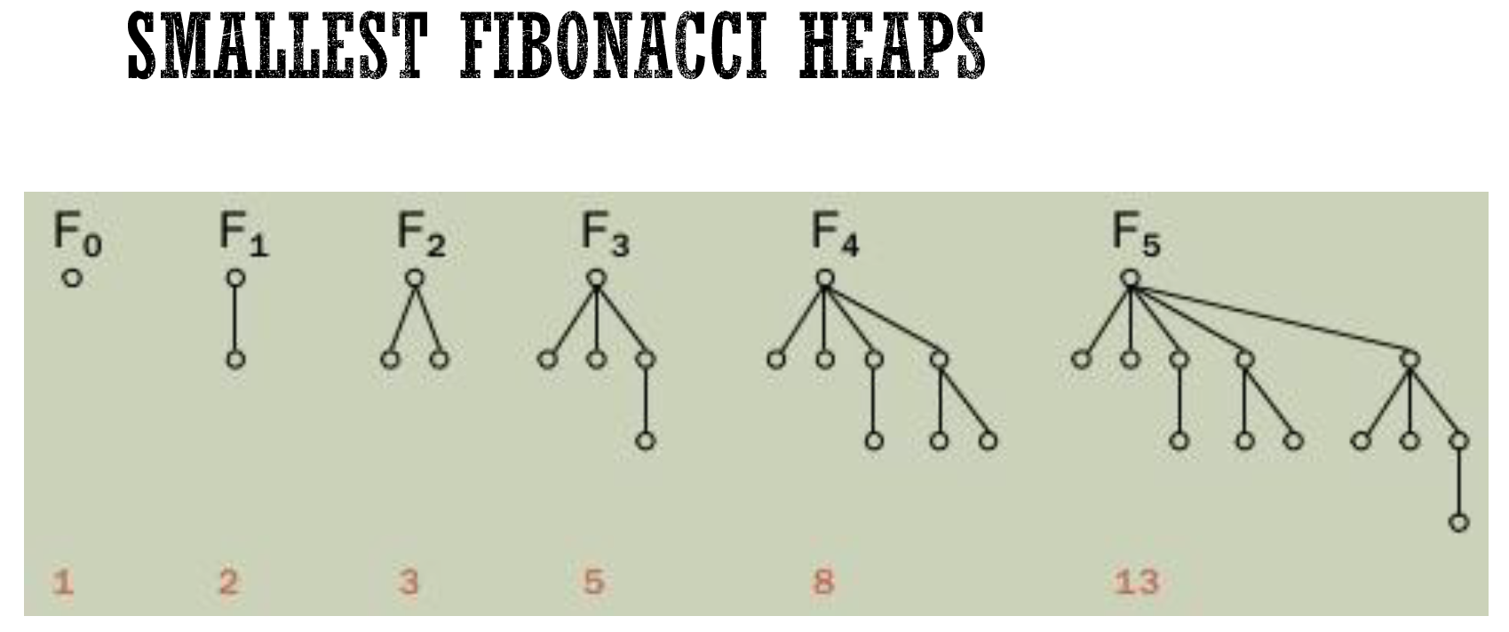
- smallest Fib heap
- size n 的 Fib heap 之 max degree
- degree d 的最小 Fib heap
Disjoint Set
also called Union-Find
https://leetcode.com/explore/learn/card/graph/618/disjoint-set/3881/
Implementation
methods:
- find: find the root of a key
- union: unite the sets of the 2 keys
implementations:
- quick find: in the array, store each's root node
- \(O(1)\) find
- \(O(N)\) union
- merge y's tree into x by setting the root of all y's tree's nodes to x's root
- quick union: in the array, store node's parent
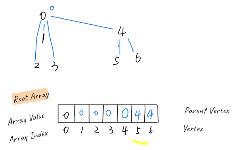
- \(O(N)\) find
- \(O(N)\) union
- merge y's tree into x by setting the parent of all y's root to x's root
- union by rank: quick union but always move short tree under tall tree when doing union
- \(O(\log N)\) find
- \(O(\log N)\) union
Quick Find:
class UnionFind:
    def __init__(self, size):
        self.root = [i for i in range(size)]

    def find(self, x): # O(1)
        return self.root[x]

    def union(self, x, y): # O(N)
        rootX = self.find(x)
        rootY = self.find(y)
        if rootX == rootY:
            return
        for i in range(len(self.root)):
            if self.root[i] == rootY:
                self.root[i] = rootX

    def is_connected(self, x, y):
        return self.find(x) == self.find(y)
Quick Union:
class UnionFind:
    def __init__(self, size):
        self.parent = [i for i in range(size)]

    def find(self, x): # O(N)
        while x != self.parent[x]:
            x = self.parent[x]
        return x

    def find(self, x): # recursive version with path compression
        if x == self.parent[x]:
            return x
        # set all the node's parent along the way to root
        self.parent[x] = self.find(self.parent[x])
        return self.parent[x]

    def union(self, x, y): # O(N)
        rootX = self.find(x)
        rootY = self.find(y)
        if rootX == rootY:
            return
        self.parent[rootY] = rootX

    def is_connected(self, x, y): # O(N)
        return self.find(x) == self.find(y)
Union by Rank:
class UnionFind:
    def __init__(self, size):
        self.parent = [i for i in range(size)]
        self.rank = [1] * size

    def find(self, x):
        if x == self.parent[x]:
            return x
        self.parent[x] = self.find(self.parent[x])
        return self.parent[x]

    def union(self, x, y):
        rootX = self.find(x)
        rootY = self.find(y)
        if rootX == rootY:
            return
        if self.rank[rootX] > self.rank[rootY]:
            self.parent[rootY] = rootX
        elif self.rank[rootX] < self.rank[rootY]:
            self.parent[rootX] = rootY
        else:
            self.parent[rootY] = rootX
            self.rank[rootX] += 1

    def connected(self, x, y):
        return self.find(x) == self.find(y)
Introduction
- equivalence relation
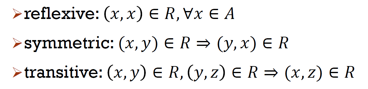
- 房間是否連通,是 equilavence relation
- x 跟自己連通
- x 連 y → y 連 X
- x 連 y 且 y 連 z → x 連 z
- 一個 set 裡面都互相連通
- 不同 set 間完全不相連
- name of set
- 其中一個元素
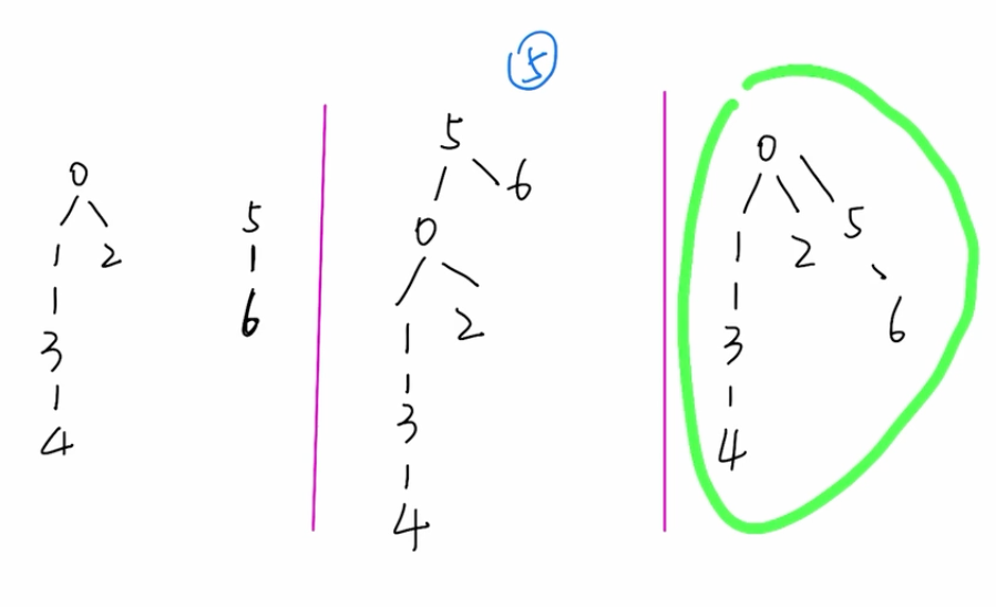
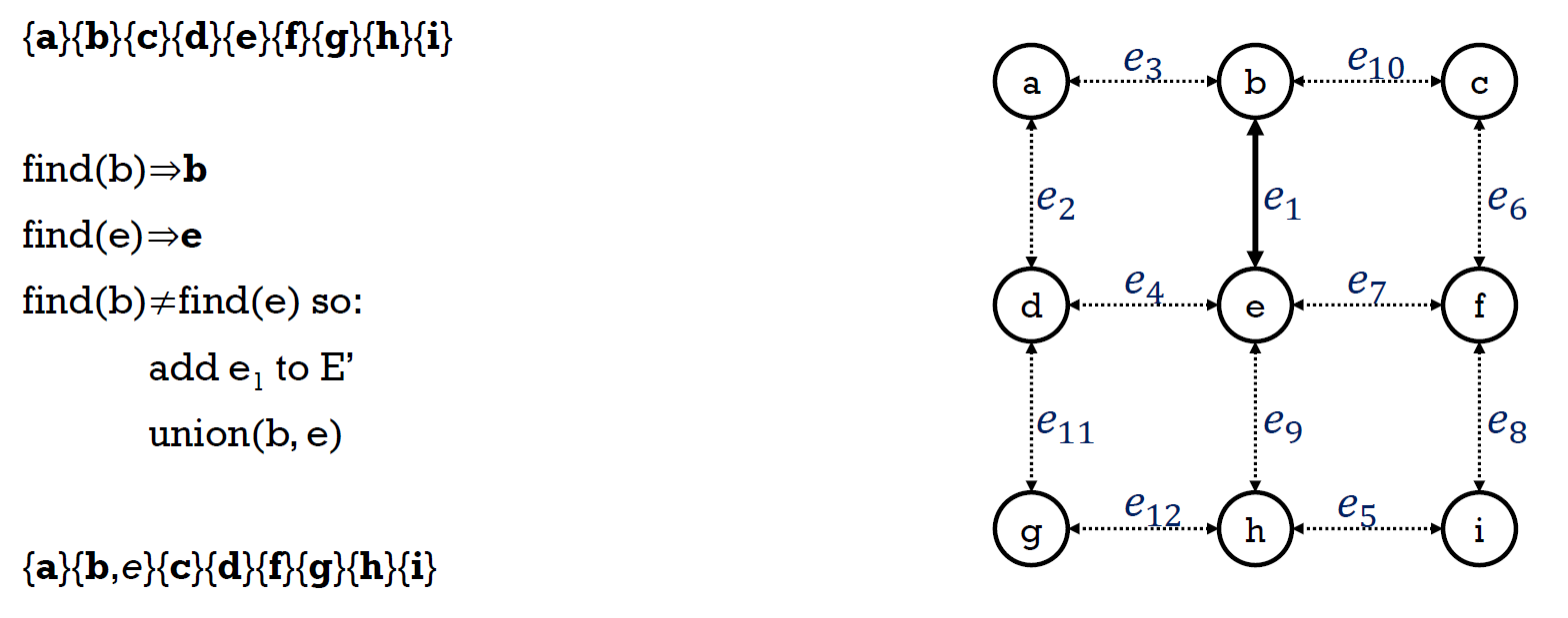
- union
- 連兩個元素 → 連兩個元素所屬的 set
- 步驟
- 找兩個元素
- find 的過程就把經過的全部指到 root
- 看這兩個元素的 root 是否一樣
- if 不一樣 → 一個 root 接到另一個 root 下,變一個 up-tree
- 結果
- 任兩 node 都互通,且只有一條路徑
- e.g.
- up-tree
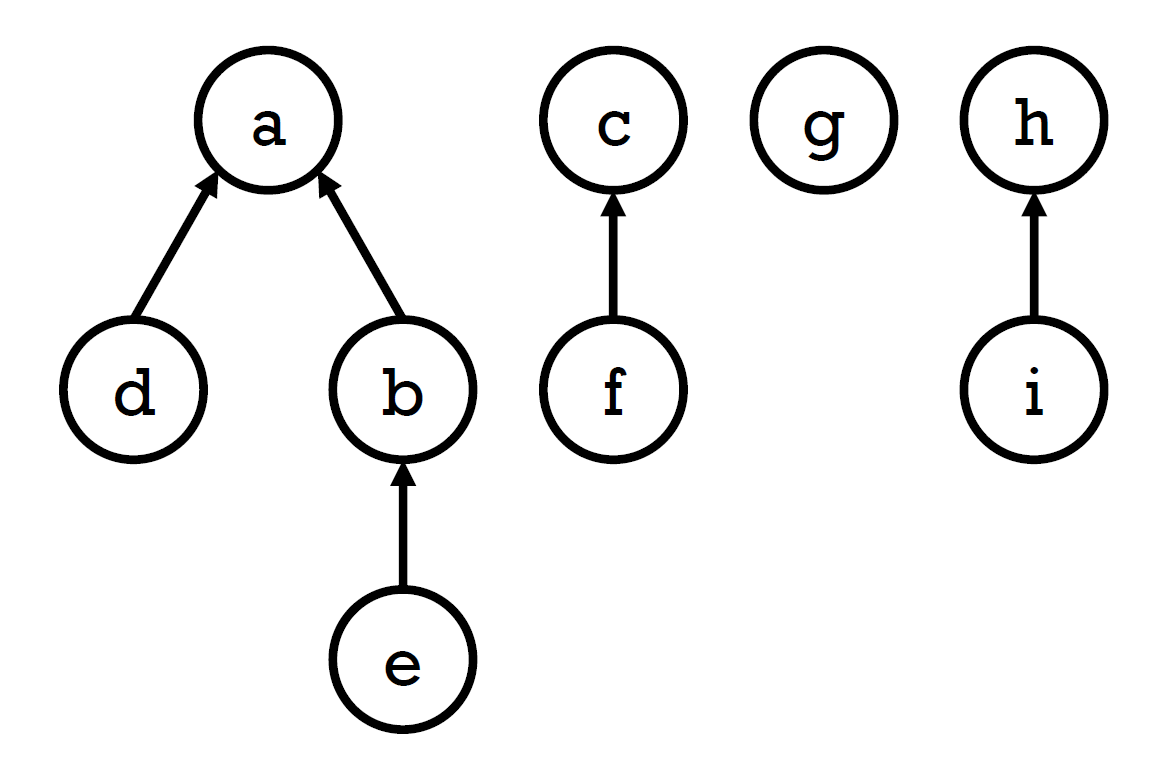
- root 為這個 disjoint set 的代表
- implementation
- array
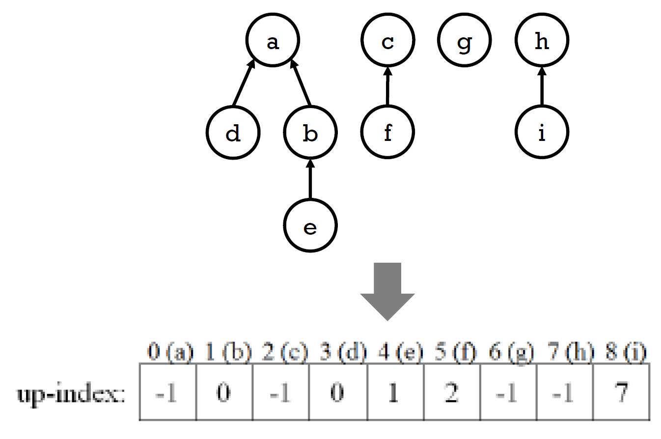
- 存 root 的 index
- 自己是 root → -1
- weighted union
- 把小的 tree 接在大的下面 s.t. 不會太深
- height h → min \(2^h\) nodes
- a tree with h=k+1 must be formed by 2 trees with h=k
- h=k + h=k-1 → h=k
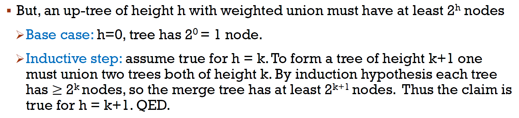
- \(h \leq log_2n\)
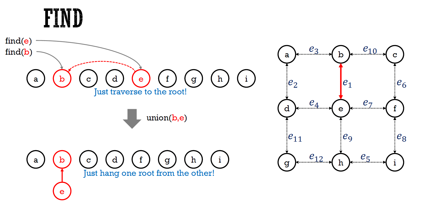
- find
- O(max height) = O(\(log_2n\))
- intuition
- find,就順便接起來節省未來時間
- ranked union
- initial rank = 0
- union 時比 root 的 rank
- rank 小者接到大者下,大者 root rank 不變
- rank 相同 →
p[x] = y,r(y) += 1
- 要創造 rank=k+1 的 root,需要 2 個 rank=k 的
- rank r → 底下 min \(2^r\) nodes
- \(rank \leq log_2r\)
- 證法同 weighted union
- parent rank > child rank
- x y 相同 rank → x y 不可能為直系血親 → x y 的 descendents 不可能有交集 → 最多有 \(\frac{n}{2^r}\) 個 rank=r 的 nodes (rank lemma)
path compression
- 把一路經過的都直接指到 root
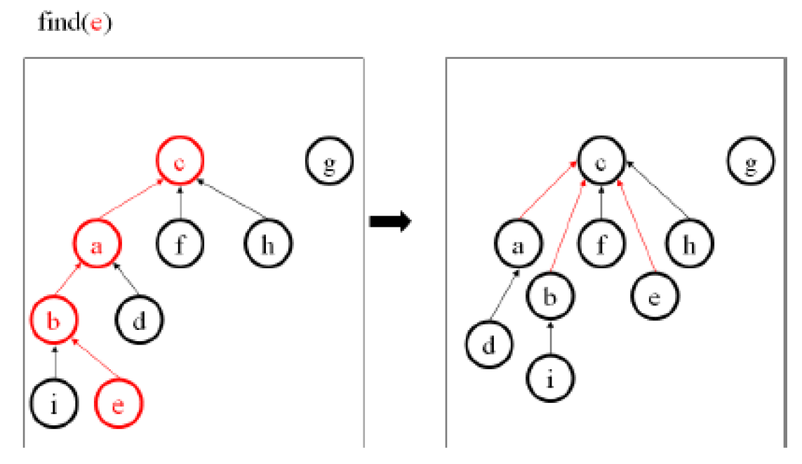
- method
- use union by rank
- find-set(x)
- if x != p[x] i.e. x 不是 root
- p[x] = find-set(p[x]) i.e. 把 x 的 parent 改為 recursive 往上找後得到的 x 的 root → 所有經過的 nodes 都直接接到 root 底下
- m 個 find's time complexity with path compression \(O((m+n)log^*n)\)
- path compression 會增大 rank gap
- x 改成直接接到 root,又 root 的 rank 比原本 parent 的 rank 大
- good & bad nodes
- good, if 符合以下其一
- x 是 root
- p[x] 是 root
- rank_block(x) < rank_block(p[x])
- 表示 rank 會跳很快
- bad, otherwise
- visit \(O(mlog^*n)\) 個 good nodes during m finds
- 最多 \(log^*n+2\in O(log^*n)\) 個 good nodes
- \(log^*n\) 個 rank block
- root
- child of root
- visit \(O(n(log^*n+1))\) 個 bad nodes
- p[x] 非 root
- rank_block(x) = rank_block(p[x])
- 共有 \(log^*n+1\) 個 rank block
- \(B_0,...,B_{log^*n}\)
- 一個 rank block 最多被 visit n 次
- 一個 rank block 裡,每個 node 最多被 visit \(2^k\) 次
- 被 visit | path compression 完,被接到 root → r(p[x]') >= r(p[x])+1 → r(p[x])+=1 at least for each operation → \(2^k\) visits 次後,p[x] 必會在更大的 rank block,x 變 good node
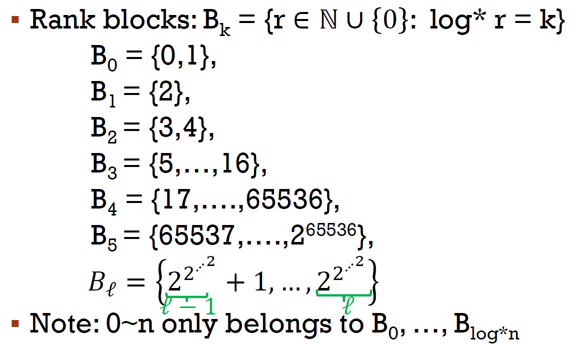
- \(B_k\) 有 \(2^k\) 個數字
- 一個 rank block 最多有 \(\displaystyle\sum_{r=k+1}^{2^k}\frac{n}{2^r}\leq\sum_{r=k+1}^{\infty}\frac{n}{2^r}=\frac{n}{2^k}\) 個 nodes
- \(B_k=\{k+1,k+2,...,2^k\}\)
- rank lemma: 最多有 \(\frac{n}{2^r}\) 個 rank=r 的 nodes
- \(log^*n\)
- = \(k\) s.t. \(log^kn\leq 1\)
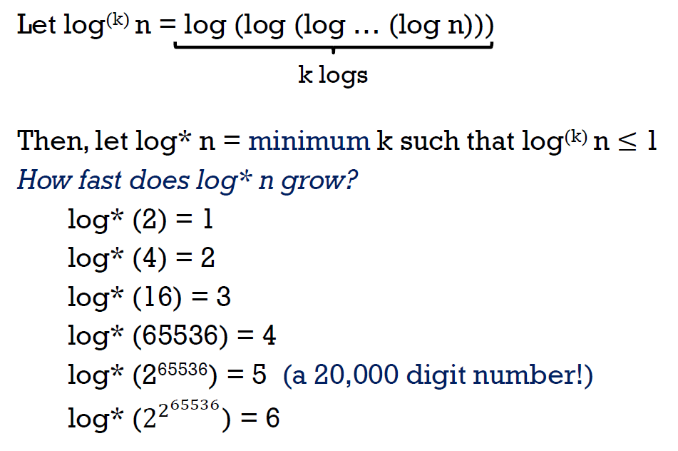
- 指 \(log_2()\)
- 成長非常慢
- rank block
- rank_block(x) = \(log^*x\)
Tarjan's analysis of path compression
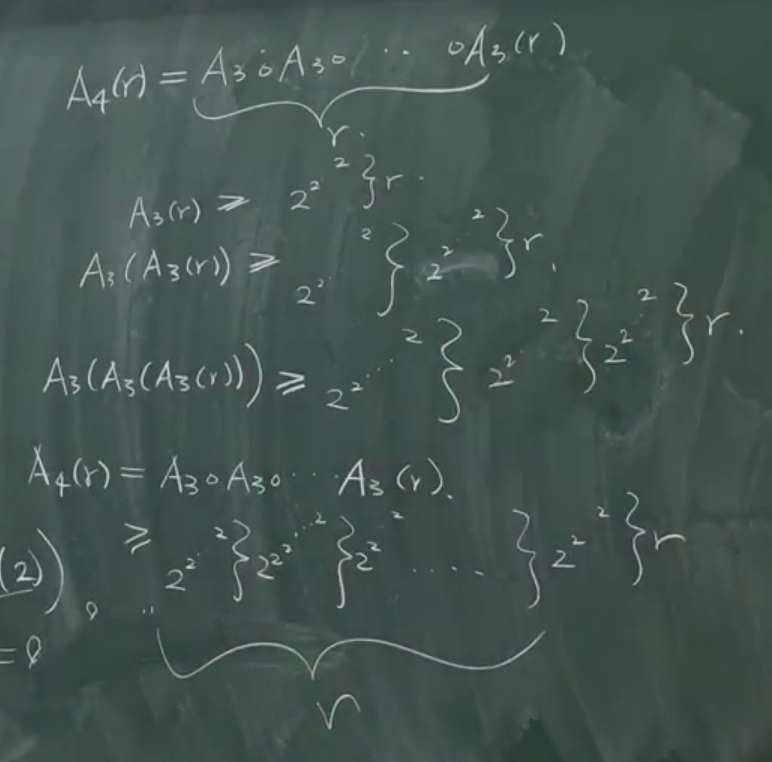
- Ackermann's function \(A_k(r)\)
- \(A_k(r)=A_{k-1}^r(r)\)
- apply \(A_{k-1}\) r times to r
- \(A_0(r)=r+1\)
- \(A_1(r)=A_0^r(r)=r+r=r\times2\)
- r += 1 做 r 次
- \(A_2(r)=A_1^r(r)=r2^r\geq2^r\)
- r *= 2 做 r 次
- \(A_3(r)=A_2^r(r)\geq2^{2^{2^{2^{.^{.^{.^{.^{.^{2^{2^r}}}}}}}}}}\geq2^{2^{2^{2^{.^{.^{.^{.^{.^{2^{2}}}}}}}}}}\) (r 個 2 的 tower)
- e.g.
- \(A_4(2)=A_3(A_3(2))=A_3(A_2(A_2(2)))=A_3(A_2(A_1(A_1(2)))))=A_3(A_2(A_1(4))))=A_3(A_2(8)))=A_3(2048))\geq\) a tower of 2048 個 2
- inverse Ackermann's function \(\alpha(n)\)
- \(\alpha(n)\) = min k s.t. \(A_k(2)\geq n\)
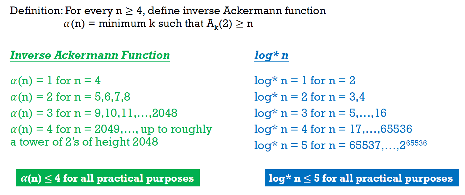
- \(\alpha\)(a tower of 2048 2s) = 4 << \(log^*\)(a tower of 2048 2s) = 2048
- rank gap \(\delta(x)\)
- \(\delta(x)\) = max k s.t. \(rank(p[x])\geq\) \(A_k(rank(x))\)
- \(\delta(x)\geq 1\) → \(r(p[x])\geq A_1(r(x))=2r(x)\)
- \(\delta(x)\geq 2\) → \(r(p[x])\geq A_2(r(x))=r(x)2^{r(x)}\)
- \(\delta(x)\geq 3\) → \(r(p[x])\geq A_3(r(x))\geq\) a tower of r(x) 2s
- \(\delta(x)\) 只會增加 but never 減少 over time
- x 若變成 non-root,則 r(x) 不再變,while r(p[x]) 可能增加
- if \(r(x)\geq2\), then \(A_{\alpha(n)}(2)\geq n\geq r(p[x])\geq A_{\delta(x)}(r(x))\) → \(\alpha(n)\geq \delta(x)\)
- \(A_{\alpha(n)}(2)\geq n\) by def of inverse Ackermann's function
- \(r(p[x])\geq A_{\delta(x)}(r(x))\) by def of rank gap
- good & bad nodes
- bad, if 以下四點同時成立
- x is not a root
- p[x] is not a root
- rank[x] >= 2
- x 有跟自己 rank gap 一樣的 非 root ancestor y
- \(\delta(x)=\delta(y)\)
- good, otherwise
- cost \(\in O((m+n)\alpha(n))\)
- cost = total visits of nodes = total visit of good nodes + total visit of bad nodes
- good visits \(\in O(m\alpha(n))\)
- bad visits \(\in O(n\alpha(n))\)
leftlist heap
- interactive visualization
https://people.ksp.sk/~kuko/gnarley-trees/Leftist.html - binary heap property
- minheap property
- 比兩個 children 大
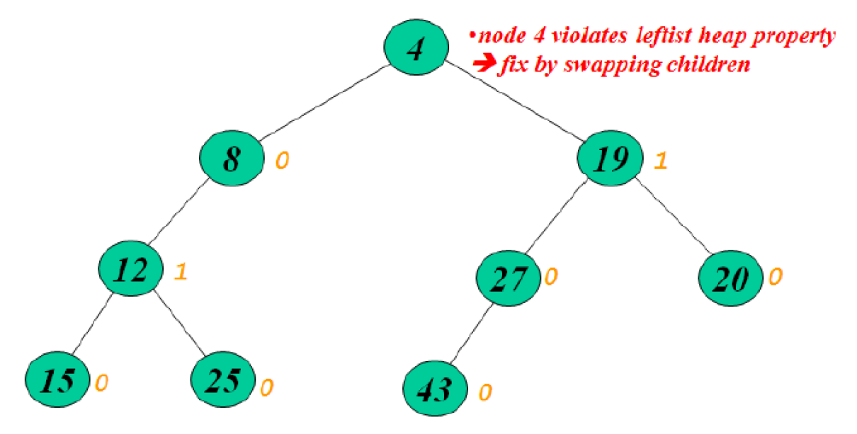
- leftheap property
- NPL(leftchild) >= NPL(rightchild)
- 違反 → swap children
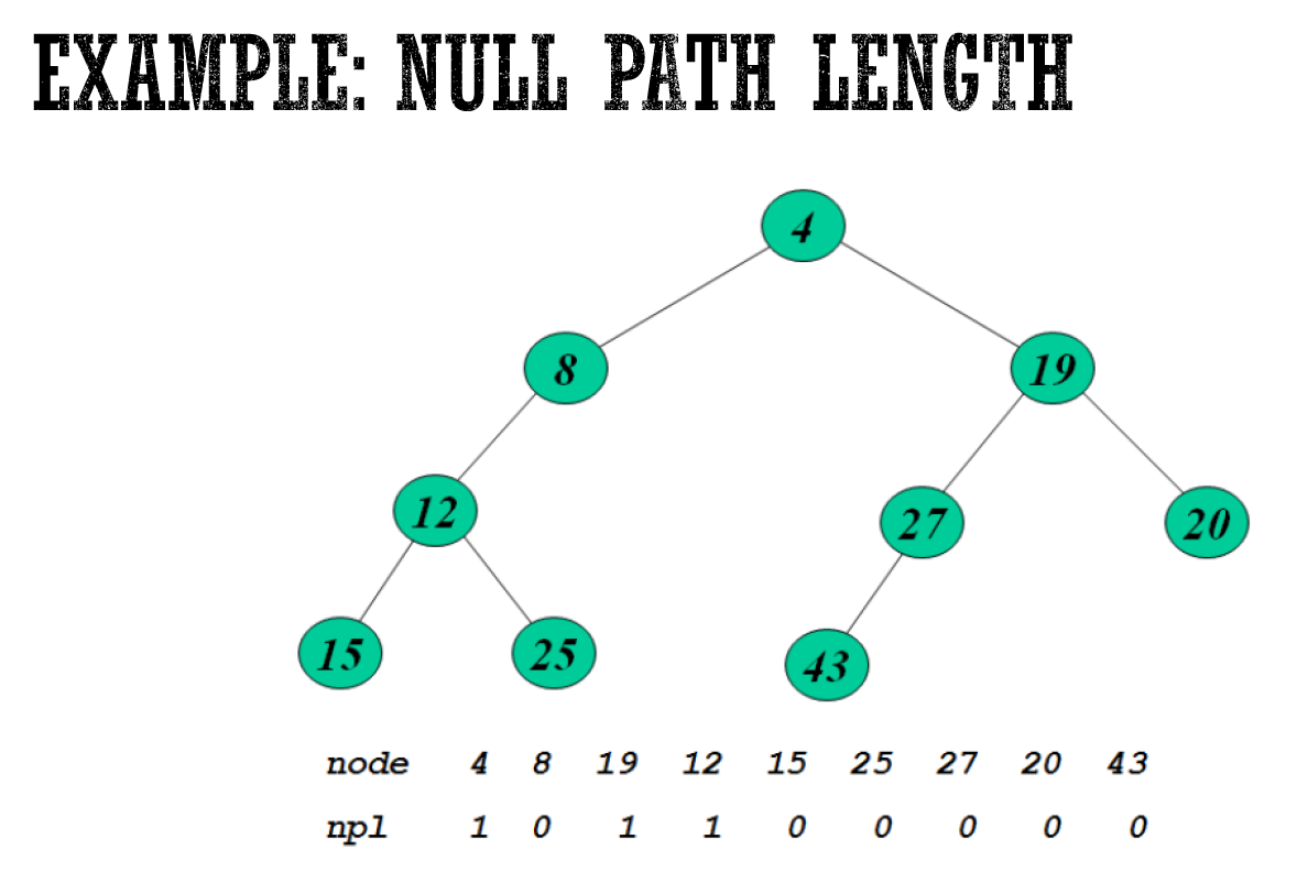
- NPL null path length
- 走到只有 0 or 1 child 的 node 的最短路徑
- 自己就是 → NPL = 0
- NPL(Null) = -1
- → only 1 child 則 left 必不為 Null
- right path 最短
- NPL(x) = NPL(x.rightchild) + 1
- x has 0 child
- 0 = -1 + 1
- x has 1 child
- 0 = -1 + 1
- x has 2 children
- NPL(x) = min(NPL(left), NPL(right)) + 1 = NPL(right) + 1
- 往右走一次,NPL -= 1
- 往左走一次,NPL -= <1
- path:走到 NPL=0 → 最短路徑:一直走 right
- pathpath
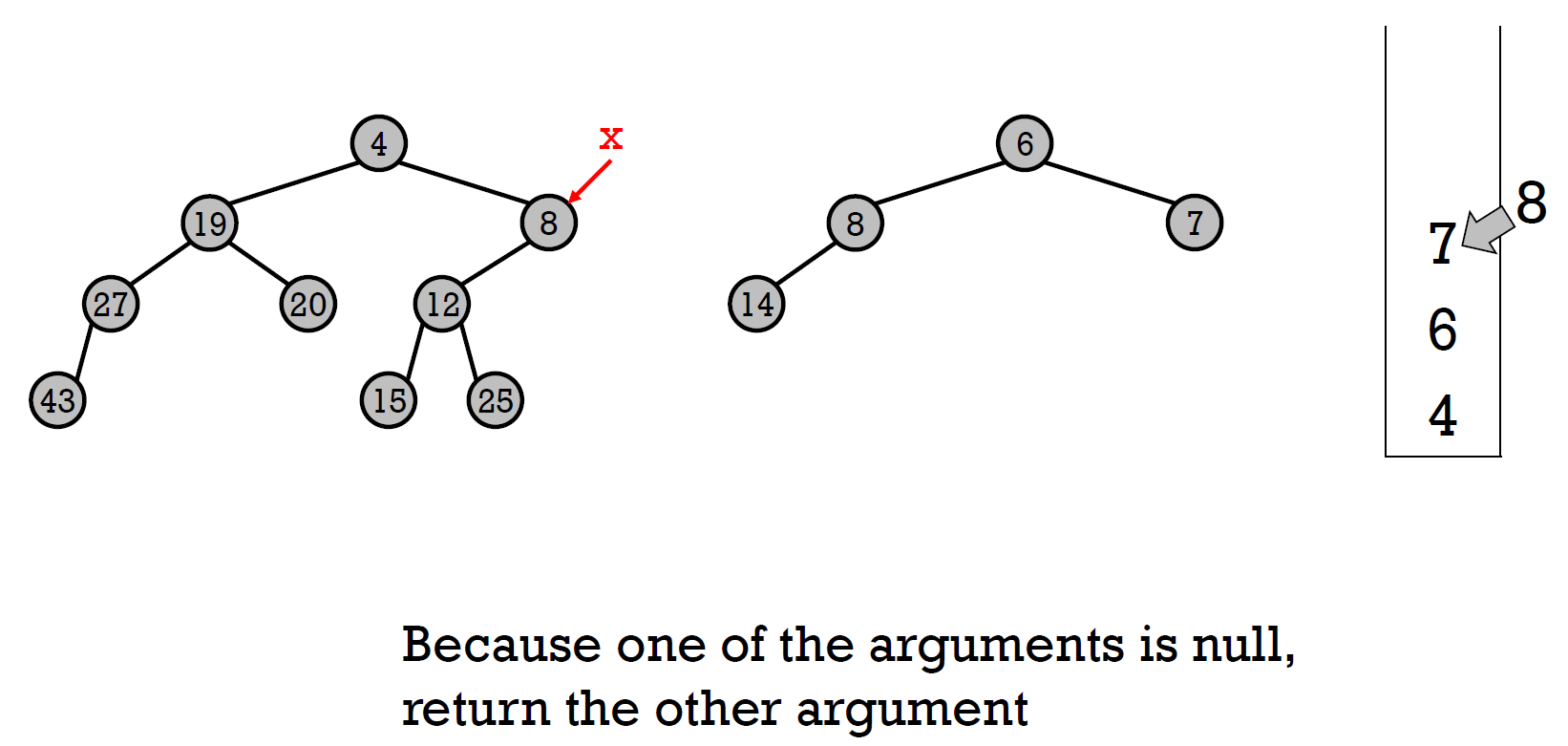
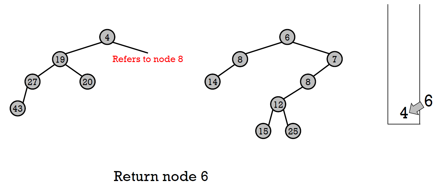
- merge
- 步驟
- x y 兩 pointer 指向兩個 root
- 比大小,較小者加進 stack,並往 right child 移動
- 重複 2.,直到一個 pointer 指向 null (假設是 y)
- y 指向 x 指向的 node
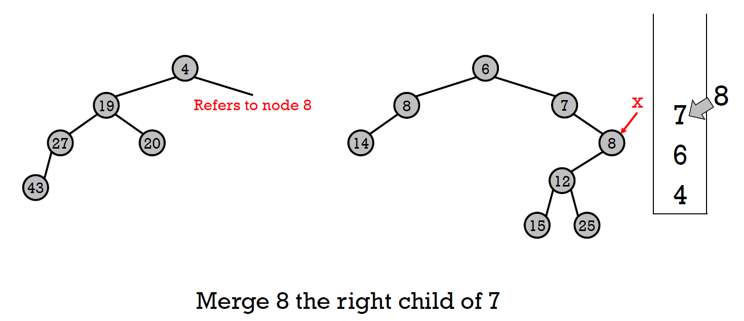
- 檢查 leftheap property, swap if needed
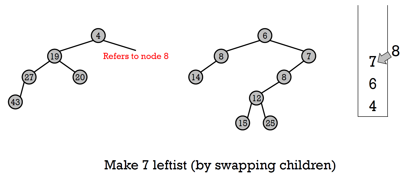
- 根據 stack,一路往回,把 node 變成上一項的 right child,並檢查 NPL
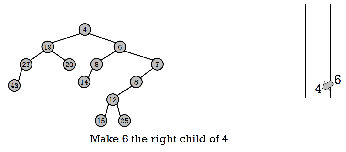
- cost \(\in O(logn)\)
- right path \(\in O(logn)\)
- 一直往 right child 走
- 會是最短的 path 因為 NPL(left)>=NPL(right)
- right path = h → 所有 path >= h → \(n\geq 2^{h+1}-1\) → \(h\leq log_2(n+1)-1\) → max num of stack \(\in O(2logn)\in O(logn)\) → cost \(\in O(logn)\)
- insertion
- merge leftlist heap with the node
- deletion
- merge left & right subheaps
- so merge, insert, delete 皆 \(\in O(logn)\)
skew heap
- interactive visualization
- binary heap property
- minheap or maxheap property
- no NPL
- so right path 不一定最短,不一定 \(\in O(logn)\)
- merge
- 跟 leftlist heap 一樣 but 根據 stack 回溯時 swap at every step
- 不判斷 NPL
- amortized cost \(\in O(logn)\)
- size = subtree 的 nodes 數
- heavy node
- \(size(x) > size(\frac{p[x]}{2})\)
- light node
- \(size(x) \leq size(\frac{p[x]}{2})\)
- 2 個 children with 1 heavy child → 另一個必為 light
- 可為 2 個 light children
- potential function \(\phi\) = num of right heavy nodes
- 根據 stack 往回走時
- 經過 light node → size *= 2 at least → 最多經過 log(n) 個 light nodes
- size = 1 走到 size = n
- actual cost = 1
- 可能被 swap 成 heavy → \(\Delta\phi\) <= 1
- amortized cost = 1 + 1 = 2
- 經過 heavy node → right heavy node swap 成 left heavy mode
- actual cost = 1
- \(\Delta\phi\) = -1
- amortized cost = 1 - 1 = 0
- amortized cost = 2log(n) + 0 \(\in O(logn)\)
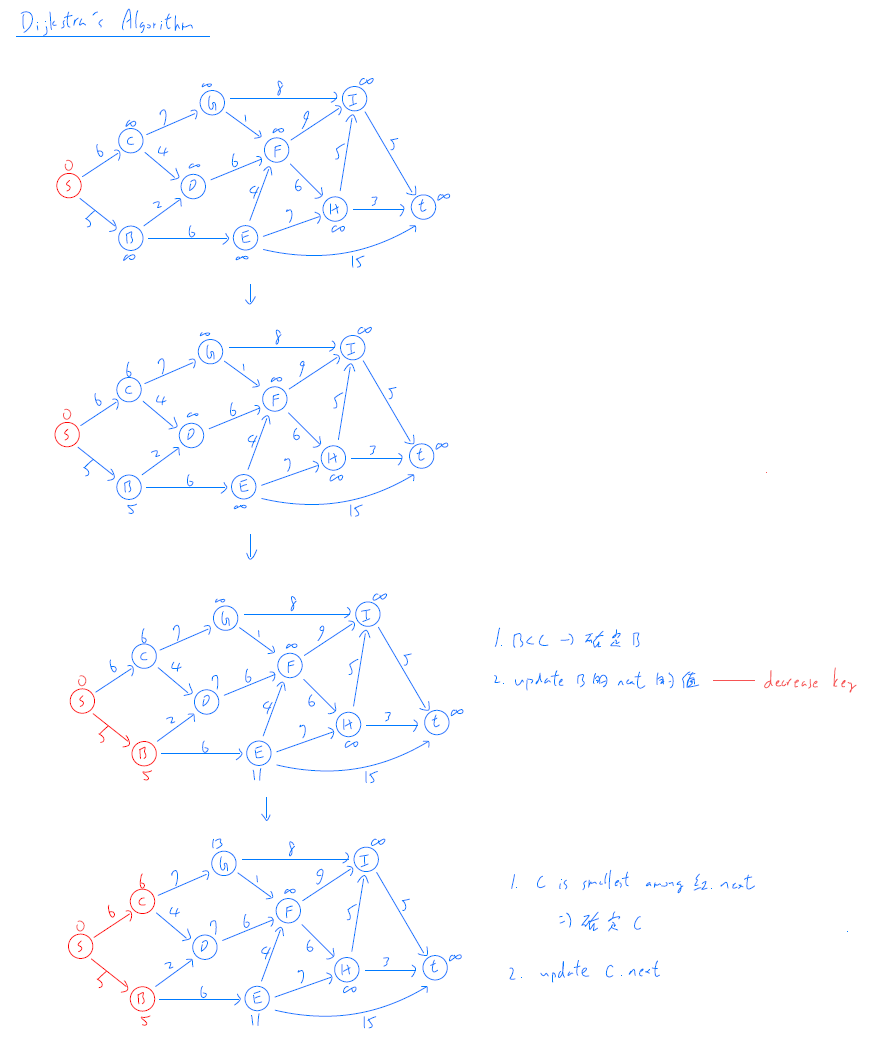
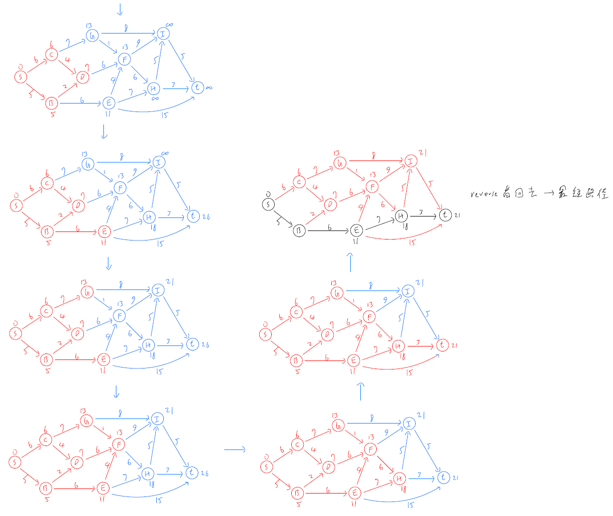
Dijkstra's Algorithm